Laser & Large Beam Profiler Q&A
Frequently Asked Questions about Laser and Large Beam Profiler systems, including our LBP-B series designed for apertures up to 800 mm.
Questions regarding product specifications and performance
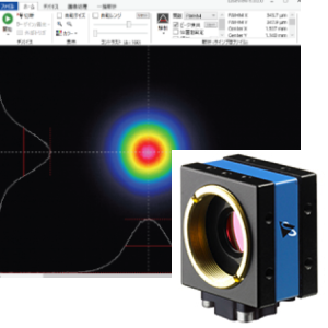
Please tell me about the laser power levels that can be used with the Laser Beam Profiler.
When performing measurements using a beam profiler, it is essential that the incident laser power remains within the permissible range for each model to avoid damaging the equipment and ensure accurate measurements. Excessive laser power input may cause sensor burnout or performance degradation.
Essential restrictions
laser power Density
The laser power density calculated based on the average output of the measurement beam must be managed to ensure it does not exceed the maximum laser power density of the equipment.
【Calculation of Average Laser Power】
Pulse energy (joules) × repetition frequency (hertz) = average power (watts)
Laser power density by model
| Model | Maximum laser power density |
|---|---|
| LBP-C series | 1 μW/cm2 (As a guideline) |
| Standard model | 100 W/cm2 |
| LBP-B series | 100 W/cm2 |
| LBP-B series | 10 kW/cm2 |
List of maximum total incident laser power by model
Keep the total incident laser power below the following value. Also, ensure that the maximum laser power density is not exceeded.
| model | Maximum total incident laser power |
|---|---|
| LBP-C series | No restrictions are imposed, but please calculate the total incident power based on the maximum laser power density specified above. |
| Standard model | 10 W |
| LBP-B series | 10 W |
| LBP-B series | 10 W |
Precautions for continuous use(LBP-B series)
Ensure the image sensor (camera) does not exceed 45°C. If the image sensor (camera) exceeds its operating temperature range (maximum 45°C), normal operation cannot be guaranteed. However, immediate failure will not occur at temperatures below approximately 60°C. As long as the unit’s temperature remains below 45°C, laser power exceeding the specified levels can be incident. There are two methods to prevent temperature rise: ① Stop light incidence when the temperature rises and wait for it to decrease. ② Install an air-cooled or water-cooled cooler to force cooling. Since no temperature sensor is built-in, measure the temperature using a contact thermometer or a non-contact infrared thermometer.
Please tell me the maximum pulse energy density that can be used with the beam profiler.
The sensor of ax beam profiler may be damaged when exposed to instantaneously high energy. Pulsed lasers, in particular, tend to have high energy density because they release large amounts of energy in a very short time.
Calculation method for pulse energy
List of maximum pulse energy density by model
| Model name | Maximum pulse energy density |
|---|---|
| LBP-C series | 1 μJ/cm2 |
| Standard model | 10 mJ/cm2 |
| LBP-B series | 10 mJ/cm2 |
| LBP-B series | 100 mJ/cm2 |
Please tell me about the optical resolution of the micro-measurement optical system option.
The higher the optical resolution of a micro-measurement optical system, the finer the structures it can separate, observe, and measure. Therefore, it is a critically important performance metric for measurement optical systems handling minute objects. The optical resolution specification is calculated based on the worst-case value within the measurement wavelength range.
Calculation formula for optical resolution
0.61 × wavelength / NA = optical resolution
Optical resolution when using LBP-C05VIS-BE
0.43
400 nm-1100 nm
2μm
Therefore・・・
- Optical resolution at 190 nm=0.61 x 0.4μm/0.43=0.56 μm
- Optical resolution at 1100 nm=0.61 x 1.1μm/0.43=1.56 μm
The 2μm specification is calculated based on the worst-case value within the measurement wavelength range.
Optical resolution when using LBP-C05VIS-BE
0.4
950 nm-1700 nm
4μm
Therefore・・・
- Optical resolution at 950 nm=0.61 x 0.95μm/0.4=1.26 μm
- Optical resolution at 1700 nm=0.61 x 1.7μm/0.4=2.59 μm
The 4μm specification is calculated based on the worst-case value of the measurement wavelength.
Please tell me about the spatial resolution and measurement error of the LBP-B series.
Spatial resolution is an indicator of how finely a beam profiler’s sensor can measure the spatial intensity distribution of a laser. When selecting a beam profiler, it is important to choose a model with appropriate spatial resolution that matches the characteristics of the laser beam being measured.
Spatial resolution of LBP-B series
The spatial resolution of LBP-B series is as follows. Measurements can be performed without any problems if the beam diameter is 6 to 10 times or more the spatial resolution. A beam diameter of 10 times or more the spatial resolution is recommended.
| Model name | Spatial resolution |
|---|---|
| LBP-B25VIS-U | 50μm |
| LBP-B50VIS-U | 100μm |
| LBP-B100VIS-U | 200μm |
| LBP-B200VIS-U | 400μm |
| LBP-B800VIS-WA-U | 1200μm |
Relationship between spatial resolutionx and measurement error in the LBP-B series (Typical example)
| Actual beam diameter | Observed beam diameter(Error %) |
|---|---|
| x μm | 1.41*x μm (+41%) |
| 2*x μm | 2.34*x μm (+12%) |
| 3*x μm | 3.16*x μm (+5.4%) |
| 5*x μm | 5.10*x μm (+2.0%) |
| 10*x μm | 10.05*x μm (+0.5%) |
Please tell me about the brightness values and light intensity of the LBP-C05VIS tif file.
Regarding brightness values
The LBP-C05VIS has 8-bit mode and 10-bit mode. When images are acquired in 8-bit mode, 8-bit TIFF images are output. When images are acquired in 10-bit mode, 16-bit TIFF images are output. Regardless of the averaging count (buffer length), images are always 16-bit when averaging is enabled. CSV files output with averaging enabled contain data with averaged brightness values. When files are output, values are rounded to 16-bit integers.
Relationship between brightness value and light intensity
A beam profiler is typically used to measure optical intensity. By combining a power meter with a beam profiler, you can calculate optical intensity by dividing the power by the beam area.
Please tell me about the attenuation rate of the Kokyo attenuator set.
When measuring laser light, an attenuator set is used to reduce the risk of CCD camera damage. There are two methods for attenuating laser power: using an ND filter for light reduction, or using a beam splitter along with ND filter for light reduction.
Method using an ND filter
ND Filter Set
Model name:LBP-OP-NDFS01
- Absorption-type ND filter
- ND filter with diagonal mount
Application
- Attenuation of laser power below 100 mW
Specifications
- OD=0.1, 0.2, 0.3, 0.4, 0.5, 0.6, 1.0, 2.0, 3.0, 4.0
- Filter size: 1 inch
About OD values (Optical density)
-
The OD value is a logarithmic value of the degree of absorption. The higher the OD value, the greater the attenuation rate.
| Optical density (OD value) | Transmittance(%) | Shading rate(%) |
|---|---|---|
| 0.1 | 79% | 21% |
| 0.2 | 63% | 37% |
| 0.3 | 50% | 50% |
| 0.4 | 39% | 61% |
| 0.5 | 32% | 68% |
| 0.6 | 25% | 68% |
| 1 | 10% | 90% |
| 2 | 1% | 99% |
| 3 | 0.10% | 99.90% |
| 4 | 0.01% | 99.99% |
Method of use in combination with a beam splitter
When laser power exceeds 100 mW, absorption-type ND filters generate thermal lensing effects, necessitating the use of a beam splitter for further attenuation. At Kokyo, we offer the following three product types, differing in attenuation rate and laser wavelength compatibility.
Model name:LBP-OP-BSVIS01(Attenuating optical system set with beam splitter)
- Directly mountable on LBP-C05VIS
- Wavelength range: 350–700 nm (or 650–1010 nm)
- Power guideline: < 1 W (for S-polarized light) < 10 W (for P-polarized light)
- ND filter included: OD=1.0, 2.0, 3.0, 4.0
Application
- Attenuation of high-intensity, high-power laser light
-
Attenuation rate table (ND filter + beam splitter)
| ND filter (OD value) | P-polarized light transmittance(%) | S-polarized light transmittance(%) | P-Polarization Shading rate(%) | S-Polarization Shading rate(%) |
|---|---|---|---|---|
| None | 1% | 10% | 99% | 90% |
| 1.0 | 0.1% | 1% | 99.9% | 99% |
| 2.0 | 0.01% | 0.1% | 99.99% | 99.9% |
| 3.0 | 0.001% | 0.01% | 99.999% | 99.99% |
| 4.0 | 0.0001% | 0.001% | 99.9999% | 99.999% |
Model name:LBP-OP-BSVIS02(Attenuating optical system set with double beam splitter)
Compared to the attenuator optical system set with beam splitter (LBP-OP-BSVIS01), it offers improved attenuation performance.(< 100 W)。
- Directly mountable on LBP-C05VIS
- Wavelength range :350-700 nm(or 650-1010 nm)
- Power guideline :< 100 W(Average output)
- ND filter included :OD=1.0, 2.0, 3.0, 4.0
Application
- Attenuation of high-intensity, high-power laser light
-
Attenuation rate table (ND filter + beam splitter)
| ND filter (OD value) | Transmittance(%) | Shading rate(%) |
|---|---|---|
| none | 0.1% | 99.9% |
| 1.0 | 0.01% | 99.99% |
| 2.0 | 0.01% | 99.999% |
| 3.0 | 0.0001% | 99.9999% |
| 4.0 | 0.00001% | 99.99999% |
Model:LBP-OP-BSUV01(UV-compatible attenuating optical system set with double beam splitter)
Compared to the attenuating optical system set with double beam splitter (LBP-OP-BSVIS02), this system extends the wavelength range into the UV micro range (200–700 nm), making it effective for micro processing and semiconductor analysis. Like the LBP-OP-BSVIS02, it can withstand use up to 100 W (average power).
- Directly mountable on LBP-C05VIS
- Wavelength range :200~700 nm
- Power guideline :< 100 W(Average output)
- ND filter included:OD=1.0, 2.0, 3.0
Application
- Attenuation of High-Intensity, High-Power UV Laser Light
-
Attenuation rate table (ND filter + beam splitter)
| ND filter (OD value) | Transmittance(%) | Shading rate(%) |
|---|---|---|
| none | 0.1% | 99.9% |
| 1.0 | 0.01% | 99.99% |
| 2.0 | 0.01% | 99.999% |
| 3.0 | 0.0001% | 99.9999% |
| 4.0 | 0.00001% | 99.99999% |
Please provide the evaluation criteria and calculation formula for sensitivity non-uniformity of the LBP-B series.
The relative sensitivity (sensitivity variation) of each pixel is corrected by uniformity correction. Sensitivity non-uniformity does not change significantly with incident light intensity.
Evaluation criteria
Even after correction, non-uniformity of 20% (±10%) or less (typical value 10% (±5%) or less) remains. Therefore, we guarantee non-uniformity of 20% or less.
Calculation formula
Sensitivity non-uniformity is evaluated using binning (averaging) data with 10×10 pixels as one segment.
(Maximum value – Minimum value) ÷ Average value = Sensitivity non-uniformity
Sensitivity non-uniformity data (LBP-B200VIS typical example)
Measurement results: 8%
Please tell me the maximum laser power density and maximum pulse energy density when using the micro-measurement optical system option.
The LBP-C05DUV-BE micro-measurement optical system option includes an ND filter with an optical density of 3.0 (OD3). The LBP-C05VIS and LBP-C05NIR-BE include an ND filter with an optical density of 4.0 (OD4). The maximum laser power density and maximum pulse energy density when using the ND filter are listed below.
When not using the micro-measurement optical system option
| Model name | Maximum laser power density | Maximum pulse energy density |
|---|---|---|
| LBP-C05DUV-BE | 1 μW/cm2 | 1 μJ/cm2 |
| LBP-C05VIS | 1 μW/cm2 | 1 μJ/cm2 |
| LBP-C05NIR-1X | 1 μW/cm2 | 1 μJ/cm2 |
When using the micro-measurement optical system option
| Model name | Maximum laser power density | Maximum pulse energy density |
|---|---|---|
| LBP-C05DUV-BE | 0.9 W/cm2 | 0.9 J/cm2 |
| LBP-C05VIS-BE | 13.7 W/cm2 | 13.7 J/cm2 |
| LBP-C05NIR-BE | 13.0 W/cm2 | 13.0 J/cm2 |
Calculation method
As the magnification of the optical system increases, the beam diameter on the sensor becomes larger, causing the power density to decrease by a factor of 1/(magnification squared).
LBP-C05DUV-BE
With a magnification of 30x and an ND filter OD3 (transmittance 0.1%),
Light intensity = 1/(30²) × 10⁻³ = 1.1 × 10⁻³
Maximum laser power density = 1 μW/cm² × 30²/10⁻³≒0.9 W/cm²
Maximum pulse energy density = 1 μJ/cm² × 30²/10⁻³≒0.9 J/cm²
LBP-C05VIS-BE
With a magnification of 37x and an ND filter OD4 (transmittance 0.01%),
Light intensity = 1/(36²)×10⁻⁴ = 7.7×10⁻⁸
Maximum laser power density = 1 μW/cm² × 37²/10⁻⁴≒ 13.7 W/cm2
Maximum pulse energy density = 1 μJ/cm2 × 37²/10⁻⁴≒ 13.7 J/cm2
Questions regarding product operation and settings
Please tell me the measurement position for the beam profile.
To verify the beam profile at a distance L from the light source, position the profiler using the following values as a reference.
When using the LBP-B series
| Model name | Distance from the front of the enclosure |
|---|---|
| LBP-B25VIS-U | 4.5±0.5 mm |
| LBP-B50VIS-U | 4.5±0.5 mm |
| LBP-B100VIS-U | 5.0±0.5 mm |
| LBP-B100VIS-WA | 5.0±0.5 mm |
| LBP-B200VIS-U | 8.0±0.5 mm |
When using the LBP-C05VIS
| Model name | Distance from the entire enclosure surface (Flange back) |
|---|---|
| LBP-C05VIS | 17.5 mm |
Please tell me how to capture images using a beam profiler along with a pulsed light source.
This is an important function for accurately capturing the beam profile of each pulse from a pulsed laser. Several methods can be used to achieve this, depending on the beam profiler model, software, and the control method of the pulsed light source. The method for synchronizing with the pulsed light source is as follows.
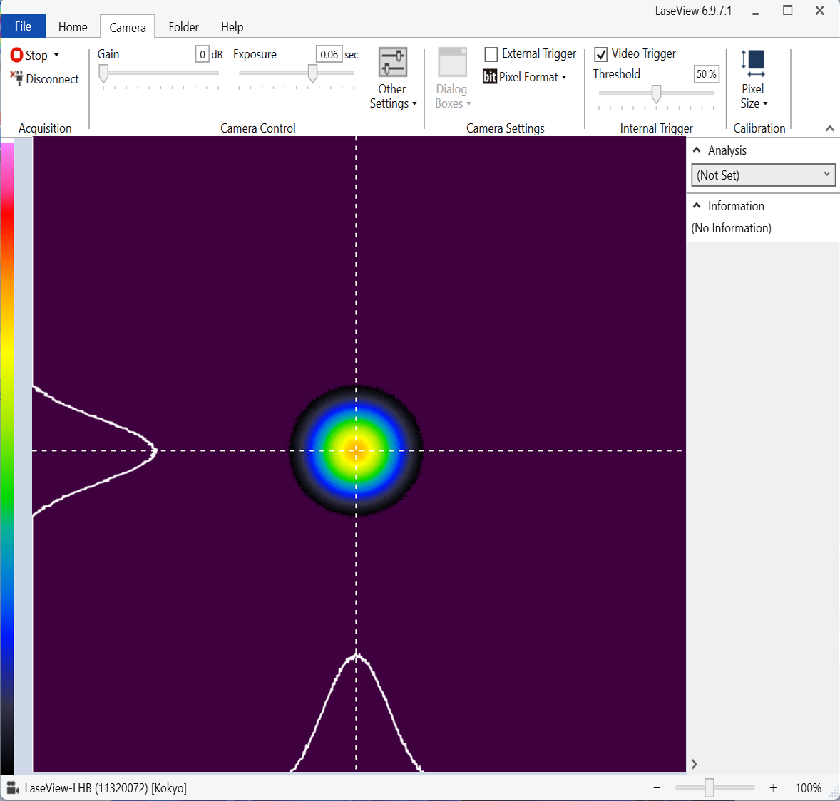
For LBP-C05VIS:
Inputting a 5–24V pulse signal to the BNC connector enables exposure synchronized to the pulse’s rising edge. Checking the box under “Camera” tab → “Camera Settings” → “External Trigger” enables the external trigger.
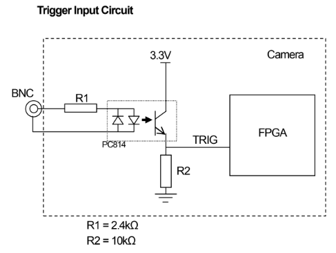
For LBP-B series
Pins 11 (+) and 12 (-) are the trigger input terminals. Apply a pulse voltage of 3.3 to 24 V with a pulse width of 10 μs or longer to the input terminals.
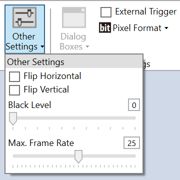
Please tell me how to adjust the camera’s black level of the LHB-B.
Black level is an offset value for brightness. Increasing the black level raises the brightness value (noise floor) in dark environments.
How to adjust black levels
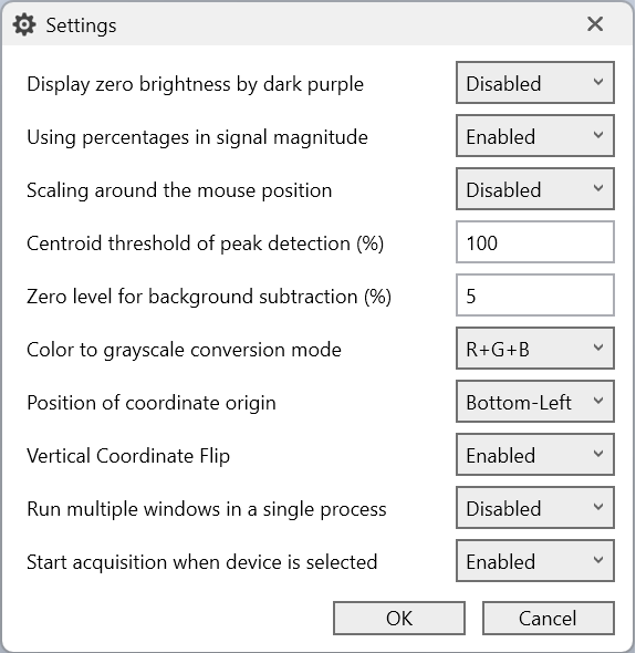
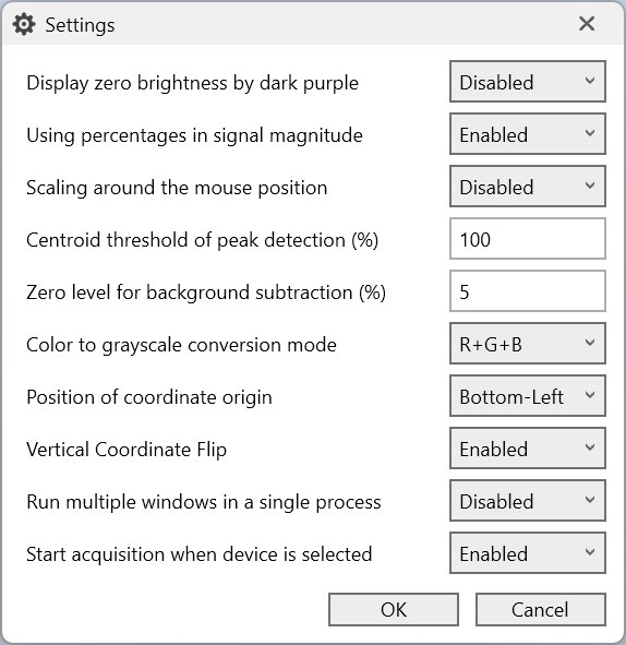
Go to “Home” → ‘Settings’ to open the settings screen, then enable “Display zero brightness by dark purple.”
When the black level is lowered to its minimum, the noise floor is clipped at zero and displayed in dark purple
This condition indicates that the black level has been lowered excessively.↓
Gradually increasing the black level causes the noise floor to approach zero, resulting in a state where deep purple and black blend together. This state represents the optimal value.↓
Note: Measurement results may vary slightly depending on the black level setting. This is because a sensitivity correction factor is multiplied by the raw brightness value.
Please advise on countermeasures for smear occurrence and gain adjustment.
In situations where smear is likely to occur, increasing the gain to ensure brightness may make the smear more noticeable.
What is a smear?:
This is a phenomenon specific to CCD cameras. A CCD converts incident light into electrical charges and outputs it as image data. When extremely bright light hits the CCD, the charges overflow, generating white streaks of noise centered on the light source in both horizontal and vertical directions. This is called smear. In CMOS cameras, incident light is amplified and converted within the pixels themselves. Therefore, no unnecessary charges are generated by principle, and smear does not occur.
Countermeasures for smear occurrence:
The sensor is saturated. Please add an ND filter or similar to reduce the light. Set the gain as low as possible and extend the exposure time to the point where the sensor does not saturate.
Note: When using the LBP-C05VIS, we recommend setting the gain to approximately 400. Below 400, the sensor may saturate before the brightness value reaches its maximum, resulting in a narrower dynamic range. This occurs because the gain setting becomes negative at gain 0. Conversely, above 400, sensitivity increases but noise also increases.
Please tell me how to use the beam profiler as an embedded device.
We can provide an API (Application Programming Interface) for customers to create programs. We only provide the function library; customers must create the programs themselves.
API positioning
This is a .NET DLL (Microsoft .NET Framework assembly) and serves as a class library that can be used by languages such as C# and Python.
System configulation
Image processing is performed using LaseView.exe, resulting in the following configuration.
Launching LaseView
On Windows, you can configure LaseView.exe to launch at startup, enabling LaseView to start simultaneously when the machine itself is powered on.
Transfer of images and analysis results
We provide functions for reading TIFF images and analysis results. A list of functions is available; please contact us if you require detailed information.
I am manually adjusting the gain and exposure time on the LBP-C05VIS, but the settings keep changing automatically.
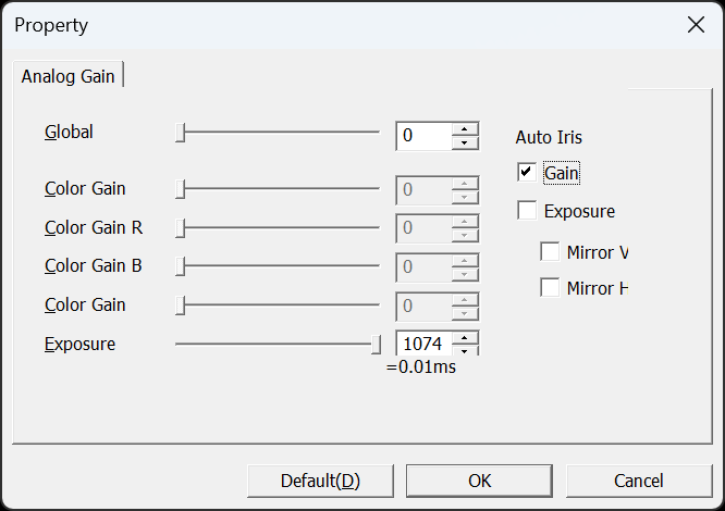
Auto Gain and Auto Exposure may be enabled. Please follow the steps below to check the auto settings.
Click the “Camera” tab → ‘Dialog’ → “Camera Settings”.
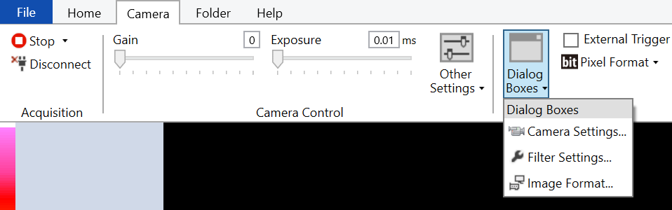
If the checkbox for Gain or Exposure under “Auto Iris” is selected, uncheck it and press OK.
How do I extend the USB cable for the LBP-B series?
The maximum cable length for USB 3.0 is specified as 3 meters in the USB standard. If a cable length exceeding 3 meters is required, we recommend the GigE model.
Introduction to the GigE Model
The following models are available; please consider them if you require a cable length of 3 meters or more.
- LBP-B50VIS-G
- LBP-B100VIS-G
- LBP-B200VIS-G
- LBP-B50NIR-G
- LBP-B100NIR-G
- LBP-B200NIR-G
- LBP-B50WB-G
- LBP-B100WB-G
- LBP-B200WB-G
What is GigE?
GigE (Gigabit Ethernet) refers to Ethernet with a communication speed of 1Gbps (1000Mbps). In addition to sending and receiving data, Ethernet includes a standard called “PoE (Power over Ethernet)” that provides power supply. GigE cameras adopt the PoE standard, enabling power delivery through a single Ethernet cable. Furthermore, Ethernet cables typically support lengths up to 100 meters, allowing for longer-distance transmission compared to USB cables.
Questions Regarding LaseView Specifications and Performance
Please tell me the PC specifications required for LaseView.
The recommended PC specifications are as follows. However, we do not guarantee operation on all computers that meet these specifications.
| OS specifications | CPU speed | Available memory | .NET Framework version | Cable connector type between enclosure and PC |
|---|---|---|---|---|
| Windows 7/8/8.1/10/11 | Intel Core i3 2GHz or equivalent or higher from another manufacturer | 512MB or more | .NET Framework 4.8 or later | PC side: USB Type A USB Micro B |
Please tell me how to save LaseView profiles as videos. Also, please tell me how to save color profiles.
About saving videos
Currently, LaseView does not have the capability to save videos in formats such as MP4. On Windows 11, screen recording can be performed using three built-in tools: Snipping Tool, Xbox Game Bar, and Microsoft Clipchamp.
Features of each tool
| Item | Snipping Tool | Xbox Game Bar | Microsoft Clipchamp |
|---|---|---|---|
| Recording range | Selected range | Only specific windows | Specific window or full screen |
| Recording microphone audio | ○ | ○ | ○ |
| Maximum recording time | 24 hours~ | 4 hours | 30 minutes |
About saving color images
From “File” → “Save Screenshot…”, you can save color images. However, images saved using this method cannot be opened and analyzed in LaseView. If you require raw data, please also save a TIFF file.
Questions regarding LaseView operation and settings
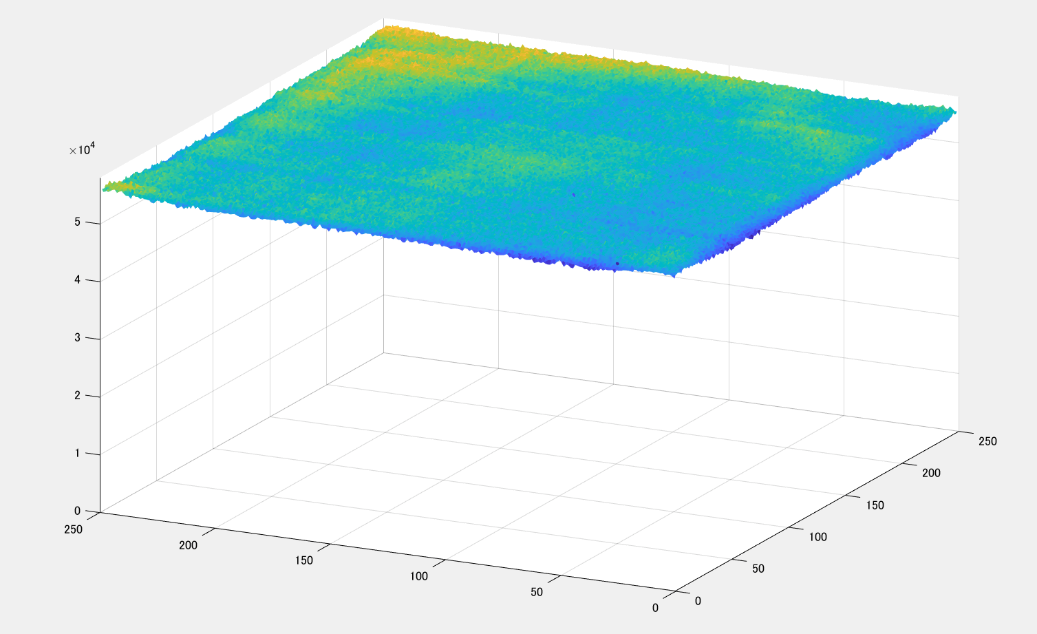
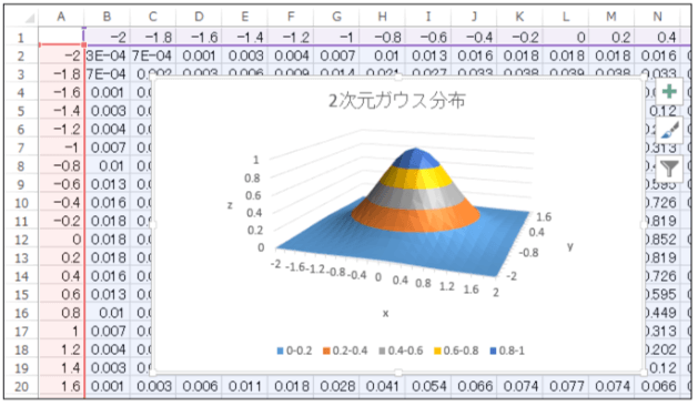
Can I create a 3D graph with LaseView?
LaseView does not have a function to display 3D graphs. In LaseView, click “File” → “Export Image” → “CSV Text”, then save the file to store the brightness values for all pixels. Processing the saved CSV file in graphing software such as Excel will allow you to create a 3D graph.
Example of 3D graph creation:
Please tell me the points to note when automatically adjusting contrast in LaseView.
Contrast adjustment does not involve adjusting the camera’s gain or similar settings; it is purely a software-based image processing function designed to enhance contrast. Automatic adjustment sets the maximum brightness value among all pixels in the image as the white level and the minimum brightness value as the black level. Below “Auto Range,” you will see a display such as “Contrast (Δ=xxxx).” This Δ value represents the difference between the white level and black level. Ensure sufficient signal strength by increasing the amount of light entering the profiler so that Δ is approximately 10000 or higher. Without increasing the light intensity, the S/N ratio will not improve.
note
During normal observation, it is recommended to fix the contrast. (reset state, auto range OFF).
Set the gain as low as possible and adjust the exposure time to prevent saturation.
Please tell me how to change the beam diameter and beam position display from pixels to micrometers or millimeters.
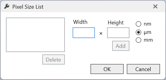
Click the “Camera” tab in LaseView → ‘Calibration’ → “Pixel Size” → “Add” to add a pixel size. The unit will change from [pixel] to [μm] or [mm].
Setup procedure
Open the “Camera” tab in LaseView → “Calibration” → “Pixel Size”. Two dropdown menus will appear: ‘Default’ and “Add…”.
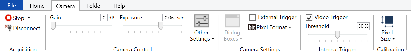
If left at the default setting, the unit of data displayed in LaseView will be [pixel].
Selecting “Add…” will display the following input screen. By selecting the display unit and entering the pixel size, the unit of data displayed in LaseView can be changed to [μm] or [mm].
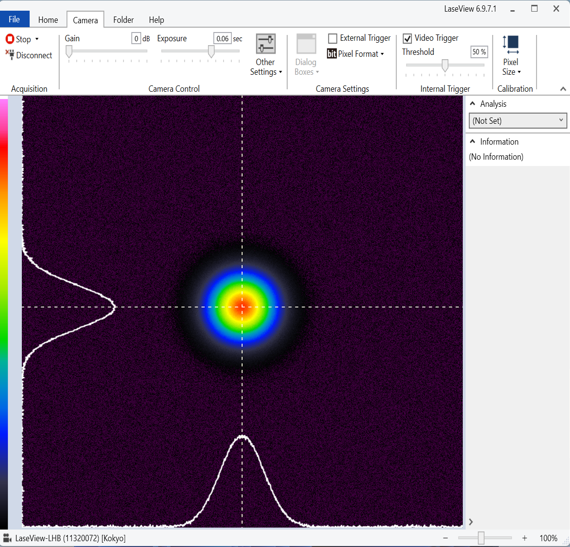
How do I check the maximum brightness value on the screen in LaseView?
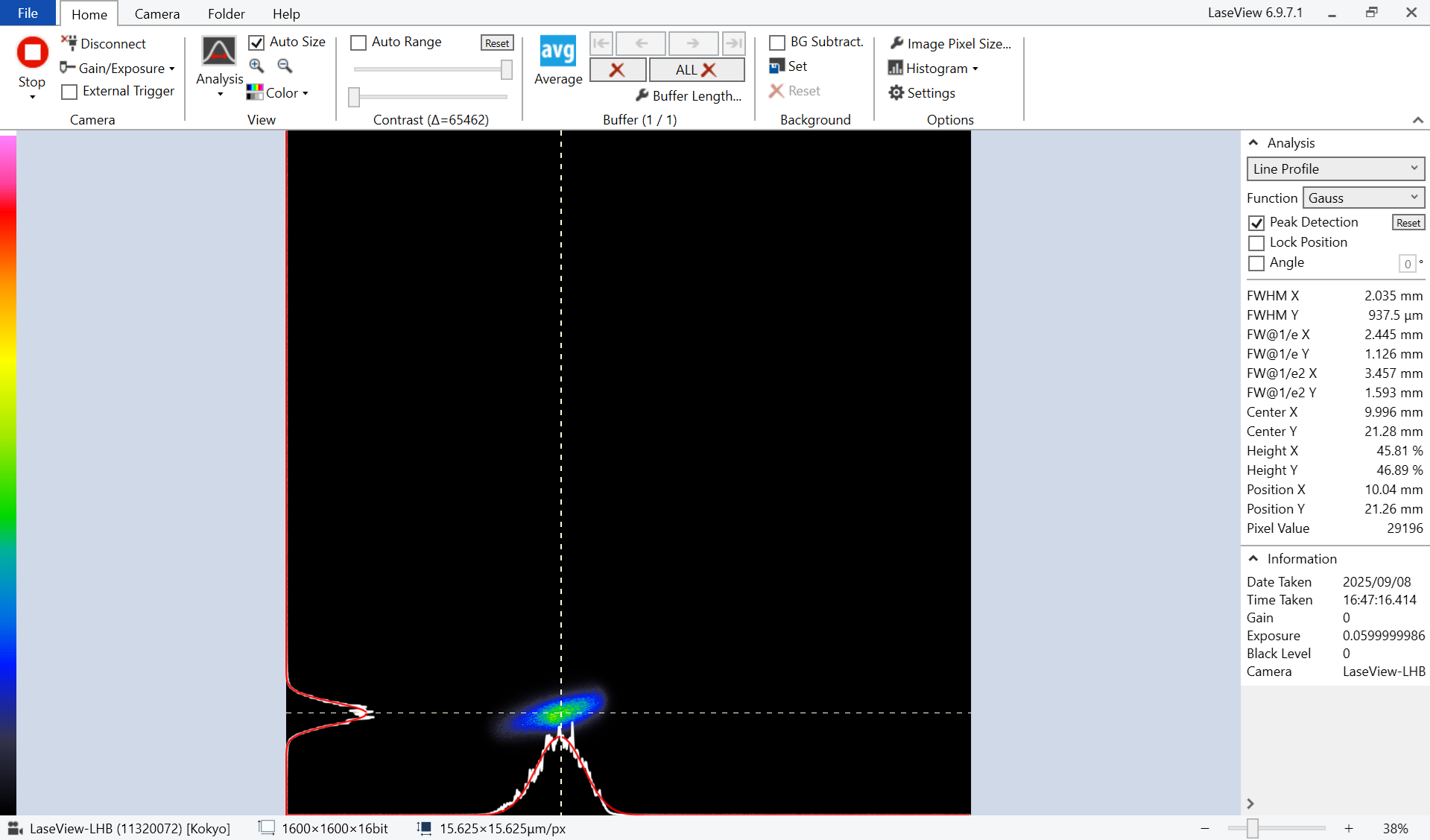
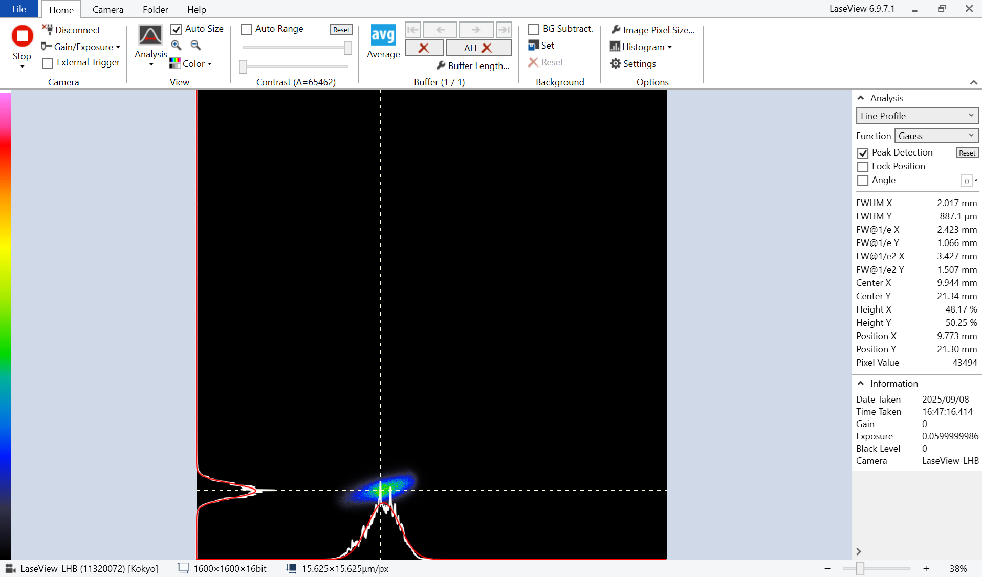
The height X and height Y values in the line profile display the maximum brightness values along the fitted profile line (e.g., Gaussian), but they cannot display the maximum brightness value within the laser beam itself. In such cases, the maximum brightness value or a brightness value close to it can be displayed using the method described below.
Display method
1. Open the settings screen via “Home” → ‘Settings’ and set the “Centroid threshold of peak detection (%)” to 100. This setting ensures that the center of gravity calculation for peak detection is performed only using pixels close to the maximum brightness value, making it easier to capture the maximum brightness value.
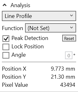
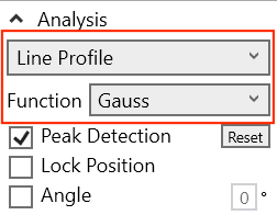
2. In “Analysis,” select “Line Profile” and turn on “Peak Detection.” At this point, the value displayed as “Pixel Value” in the analysis results will be the brightness value of the pixel where the XY profile lines intersect.
Measurement example
The following examples illustrate beam shapes with spatially non-uniform distributions, rather than clean Gaussian profiles. Setting the intensity threshold to 100% allows profile lines to be placed closer to pixels near the brightness peak.
For a strength threshold of 50%
Pixel Value 29196
When the intensity threshold is 100%
Pixel Value 43494
How do I display the center of the screen as the coordinate origin in LaseView?
By default, the top-left corner of the screen is the origin. To set the center of the screen as the origin, please configure the following settings.
How to set up
Open the settings screen from “Home” → “Settings” and set the coordinate origin to the center.

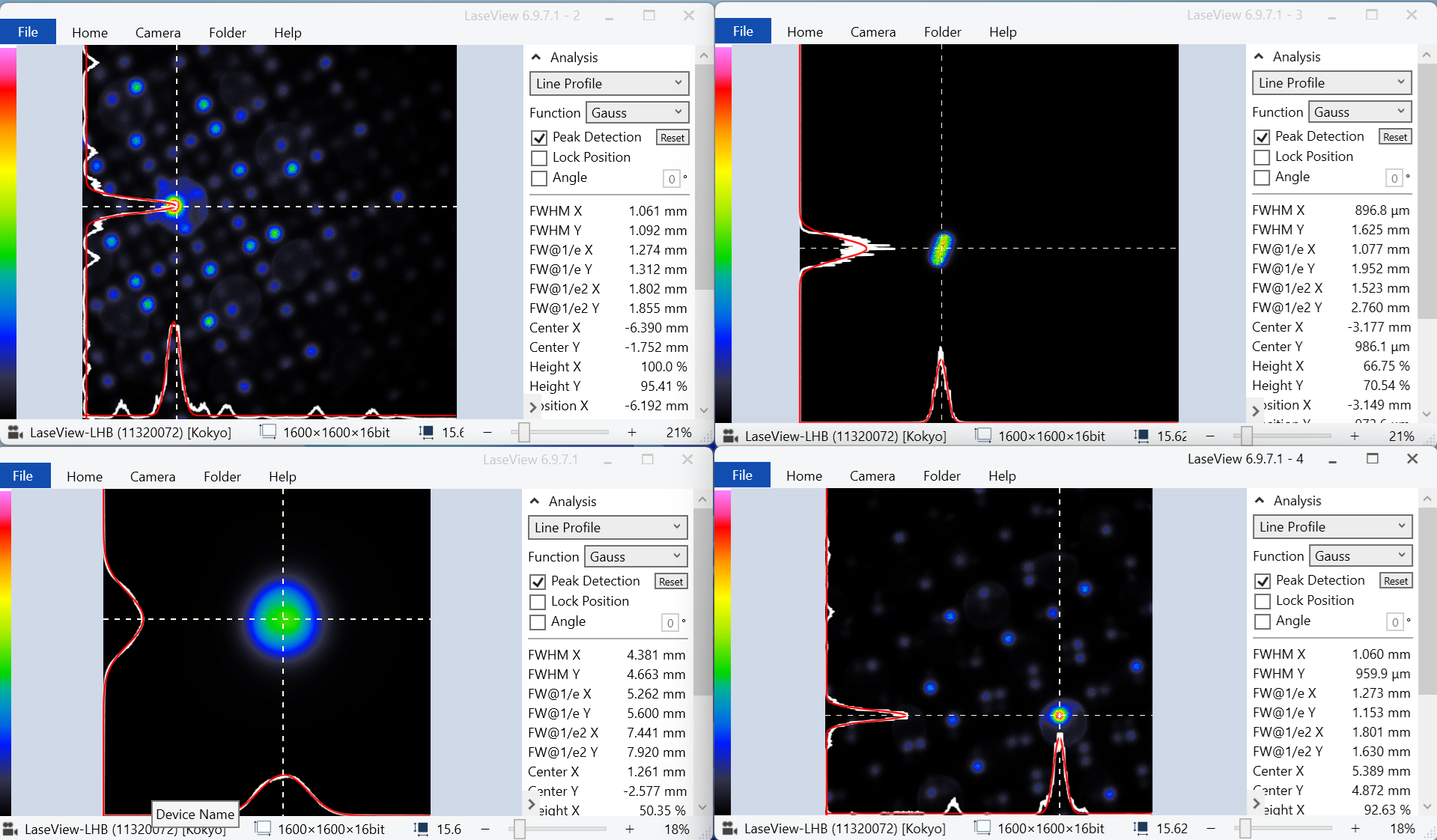
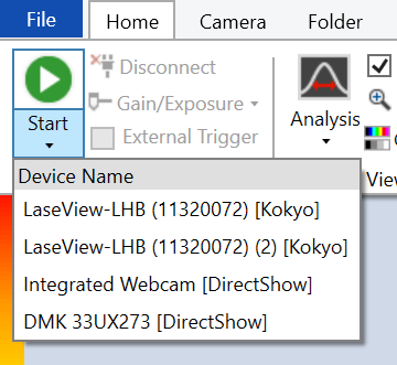
Is it possible to simultaneously view multiple cameras in LaseView?
Launching LaseView software multiple times and individually selecting the camera to use for each launched window enables simultaneous observation with multiple cameras. Furthermore, since it can capture images from commercially available cameras, simultaneous observation using multiple cameras from different manufacturers is also possible.
Observation method
This time, we will introduce an observation case using four cameras.
- Double-click the LaseView icon four times to launch the LaseView application four times.
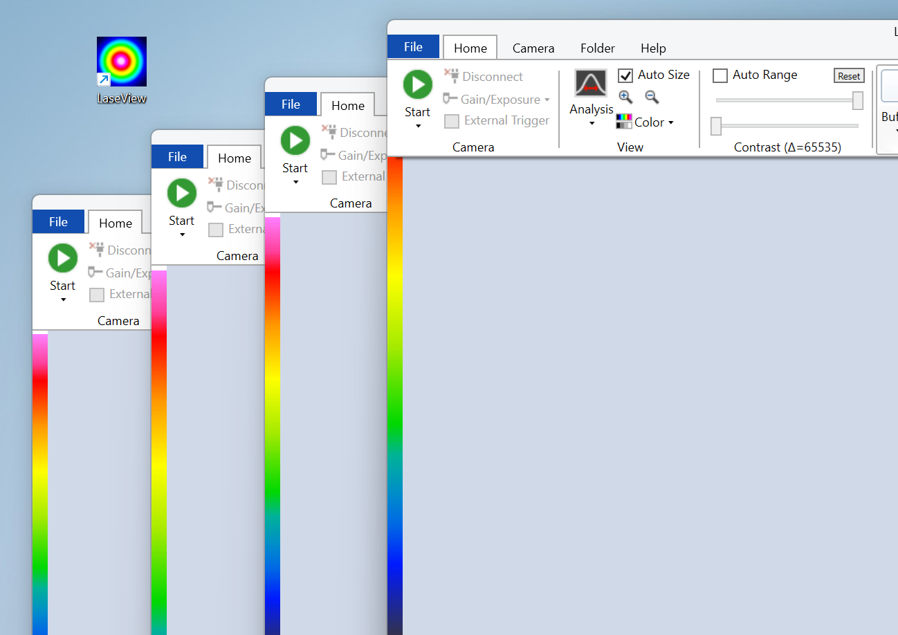
- Manually arrange the windows so that the monitor screen is divided into four sections.
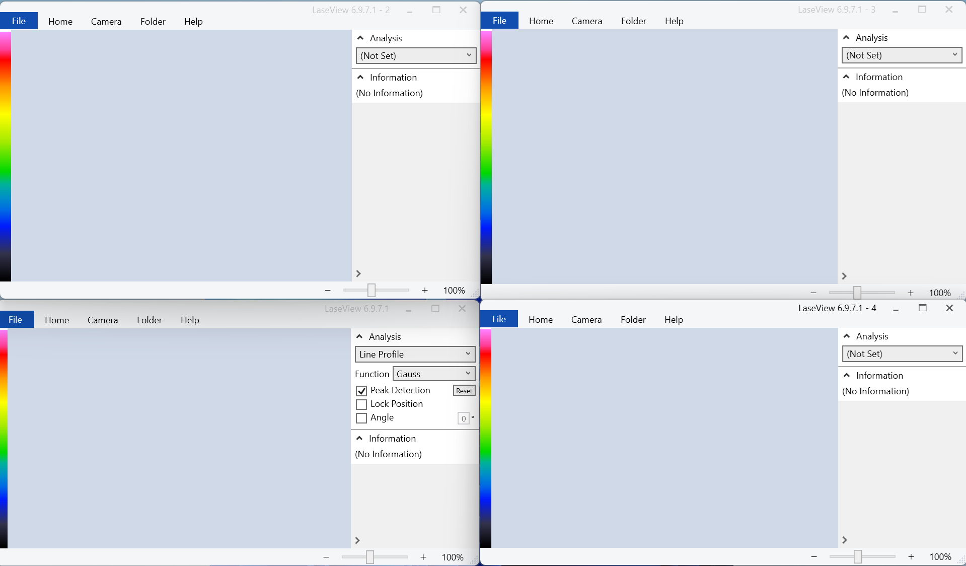
- Simply select the camera you want to display in each window from the dropdown menu, and you’re all set.
Note:Please connect multiple cameras to your PC beforehand.
How do I subtract the baseline value when measuring D4σ in LaseView?
If the baseline value is large or not subtracted from the image, the baseline value near the sensor edge is included in the D4σ integral value, causing the calculated D4σ value to be larger than the actual value. Therefore, baseline subtraction is essential for accurate D4σ measurement. When measuring D4σ, use the background subtraction function in LaseView.
How to Set Up
1. In a completely darkened environment, click the “Set” button in the background menu from the “Home” screen to register.
2. Turning on BG Subtraction enables background subtraction.
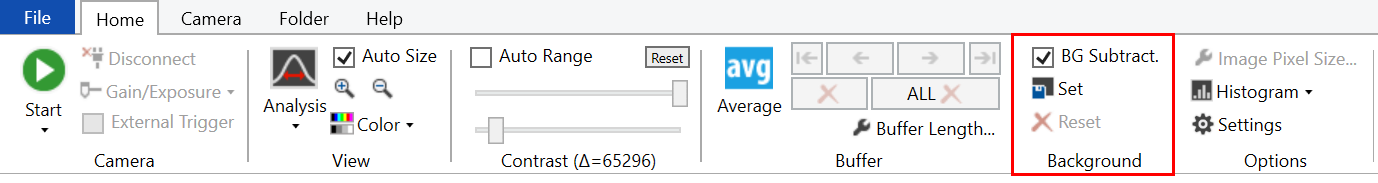
Note: If the noise floor in the dark state is sufficiently uniform, background subtraction is not particularly necessary. Even without performing background subtraction, baseline subtraction is performed correctly and accurate D4σ values are calculated.
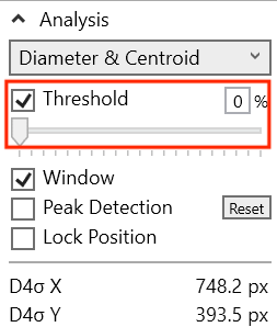
Threshold Setting
The threshold for “Diameter & Centroid” is used when changing the baseline (zero level) during integration, but it is usually fine to leave it OFF. When OFF, the baseline is set automatically.
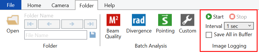
In LaseView image logging, the minimum log interval is 1 second. Please tell me how to save at a faster rate.
The image logging function allows image saving at intervals as short as 1 second. To save at intervals shorter than 1 second, use the LaseView buffer function in combination.
How to Set Up
When you check “Save All in Buffer” in the “Image Logging” function and set the logging interval to 1 second, a file containing multiple images will be generated every second, allowing you to save all captured images.
Sample Photos
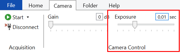
For example, setting the exposure time to 10 ms results in a frame rate of approximately 100 fps. With a log interval of 1 second and a buffer length set to 100, it is theoretically possible to save 100 images every second. However, since there is some variation in the timing of saves, setting the buffer length to the absolute minimum of 100 may result in images being missed. Please set the buffer length to a generous value, such as 200. The image logging function is designed to save only unsaved images within the buffer. Therefore, even if the buffer length is set longer, duplicate images will not be saved.
When the number of saved images is low
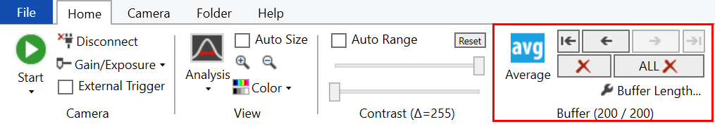
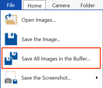
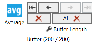
For short periods of several seconds to tens of seconds, it is possible to continuously acquire and save images using a buffer. In LaseView, the latest images are temporarily stored in memory for the number specified by the “Buffer Length…”. Using “Save All Images in the Buffer…” allows you to save multiple images as a single file (a multi-page TIFF file) containing all images in the buffer.
While there is no limit to the buffer length you can set, please note that setting an excessively long buffer length exceeding your PC’s memory capacity may cause unstable PC operation. Depending on the image size, a buffer length of 1000 or less is typically sufficient.
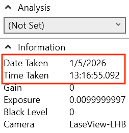
How to Check the Shooting Time
The acquisition date and time of each image, measured in milliseconds, is embedded as metadata within the image file. Using the “Buffer” UI, you can switch between displayed images and view the acquisition date and time for each image in the “Information” field.
Note: The acquisition time is the moment the image was transferred from the camera to the PC and LaseView completed buffering. Therefore, it may differ slightly from the actual time the camera began exposure. For example, when capturing images at 10fps, the acquisition time interval is not strictly 100ms and may exhibit some variation.
How can I check the beam diameter over time in LaseView?
Use LaseView’s custom features. You can measure and graph images saved using image logging or buffer functions.
How to Set Up
1. Click “Open” from the “File” menu, then select the folder where you saved the image.
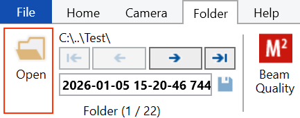
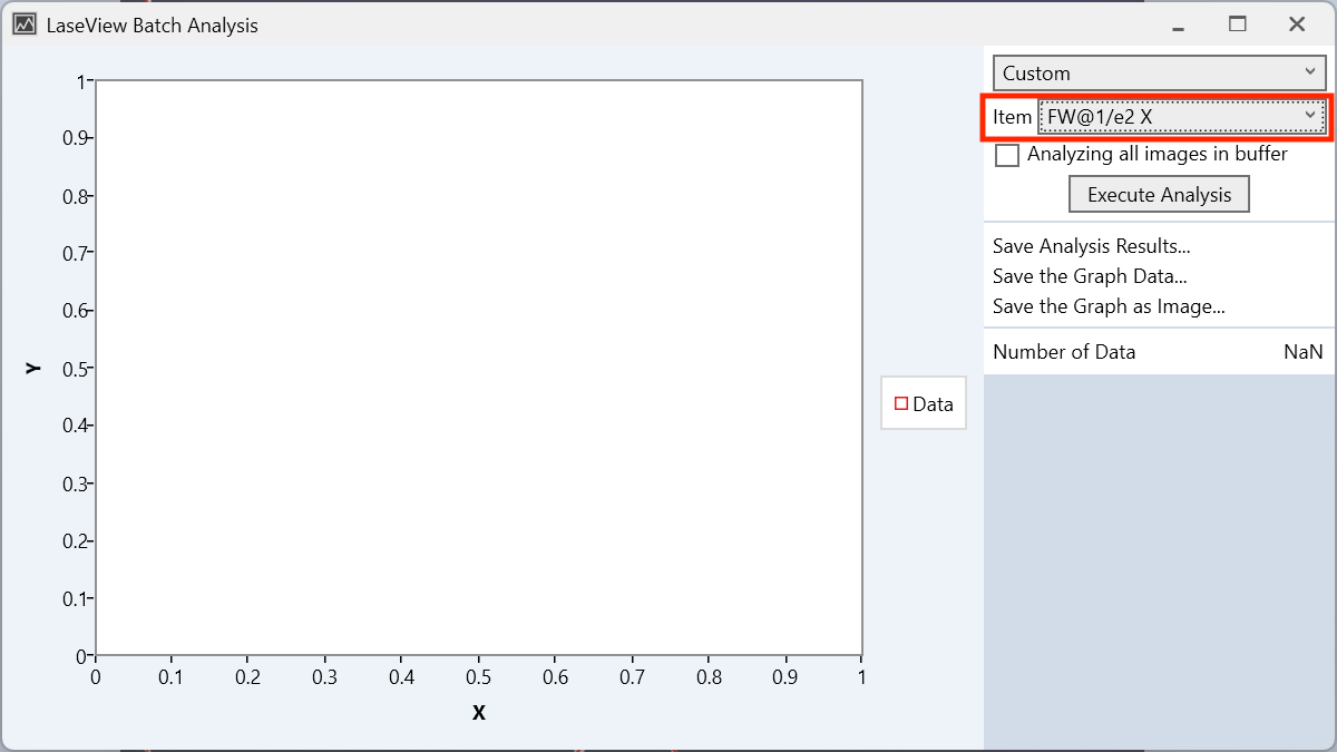
2. Click “Custom” to open the batch analysis menu.
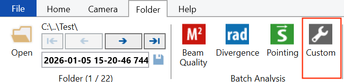
3. Select the menu you wish to analyze in advance, then choose the measurement item from the pull-down menu. In the example below, FW@1/e2 X is selected for the line profile.
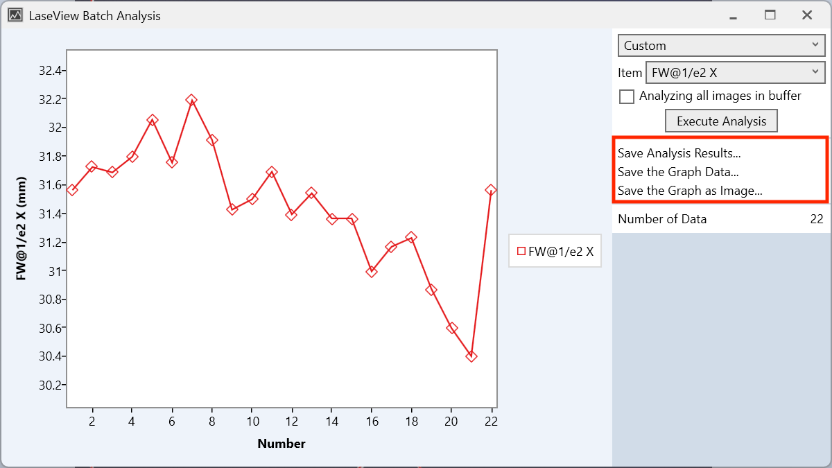
4. Click “Excute Analysis” to complete the analysis. You can save the analysis results as a CSV file or save the graph as an image.
Please explain the relationship between LaseView’s averaging function and buffer length.
LaseView’s averaging process uses images temporarily stored in the buffer for averaging. It performs averaging based on the number of images set as the buffer length.
How to Set Up
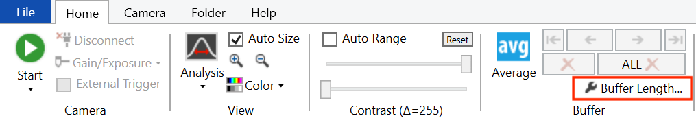
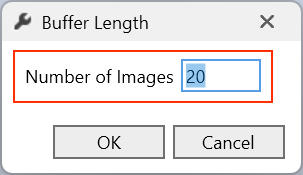
1. From the “Home” menu, click “Buffer Length…” in the buffer menu to set the number of images.
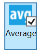
2. Click “Averaging” to enable the averaging process.
Averaging Method
Averaging is a moving average. When the number of images exceeds the buffer length setting, older images are automatically deleted sequentially.
Average time
The averaging time can be calculated using the following formula.
Number of images / Frame rate = Average time
Note: The reciprocal of the exposure time does not equal the frame rate. In practice, the frame rate is determined by the set “maximum frame rate.” If the exposure time is longer than the reciprocal of the frame rate, the actual frame rate is limited by the exposure time. In this case, the reciprocal of (exposure time + α) becomes the frame rate. +α represents the time required for image readout and transfer.
For example, with a frame rate of 100 fps and 20 images, the average time is 0.2 seconds.
20 / 100 = 0.2 sec
Update cycle
The averaging update cycle matches the frame rate. For example, at 100 fps, the update cycle is 10 ms.
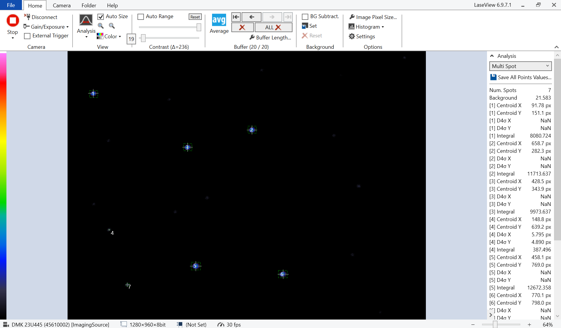
Please explain the threshold adjustment for LaseView during multi-spot measurements.
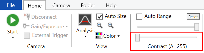
LaseView’s diameter and centroid measurements include threshold adjustment and range setting functions, but multi-spot measurements do not have a threshold adjustment function. To suppress the influence of background noise, use the contrast adjustment on the home screen. Adjusting the lower limit value under “Contrast” causes pixels below this value to be ignored, functioning as a threshold adjustment.
How to Set Up
From the “Home” menu, scroll the lower limit adjustment bar in the contrast menu with your mouse to adjust the contrast.
Before adjustment

After adjustment
Please explain the difference between line profiles and integral profiles in LaseView.
Line profiles measure luminance along horizontal or vertical lines set on the screen. In contrast, integral profiles represent the value obtained by integrating all pixels in the horizontal or vertical direction. While integral profiles are less susceptible to image noise, please note the following points.
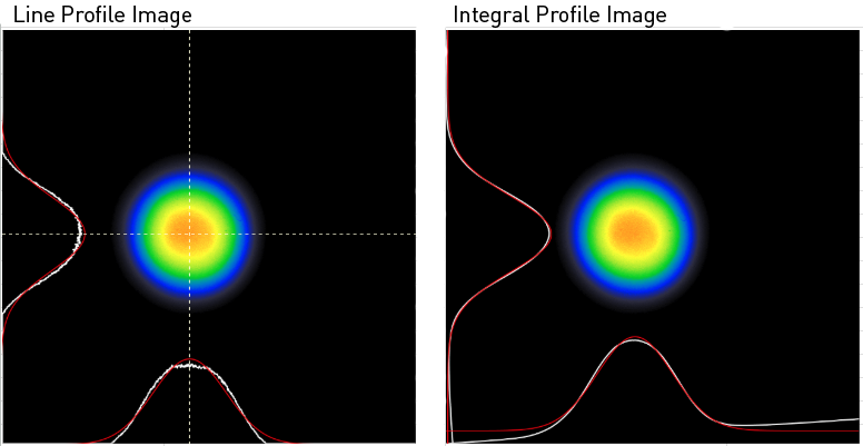
Integral Profile
The graph displayed in the “Integral Profile” shows the profile integrated along both horizontal and vertical lines. This reduces noise due to the effect of spatial averaging.
However, compared to the “Line Profile,” the beam diameter changes. The beam diameter calculated from the integrated profile generally differs from the actual beam diameter. While it can be used as an indicator of beam diameter, it is not suitable for measuring the absolute value of the beam diameter.
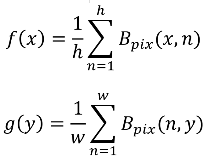
Calculation Method for Integral Profiles
The calculation method for the integral profile is as shown in the formula below. f(x) is displayed in the graph at the bottom of the screen, and g(y) is displayed in the graph on the left side of the screen. Bpix(x,y) is the luminance value of each pixel, h is the pixel height of the image, and w is the pixel width of the image.