0. FIber laser characteristics
0.1. Compact and light
Optical fiber can be made compact and light since the fiber can be rolled up. Additionally, because the laser head can be small, a flexible system up is possible. Therefore, the setup cost can be saved and the setup position can be flexibly determined.
0.2. Maintenance free
For bulk-type high-power solid-state laser, since thermal effects, such as the thermal lensing effect and the thermal birefringence effect. are remarkable, the beam quality is dramatically lowered. Therefore, when a bulk-type solid-state laser is developed, a cooling system must be carefully designed. On the other hand, the cooling system for fiber laser with 100W or less is a simple air-cooling. This is because the fiber laser is superior in the heat releasing property since [surface area/volume] of an optical fiber which is used as a laser medium is fourth-order or more larger than that of a rod-type medium in the bulk-type solid-state laser. Fig.1.27 shows schmatics of radiation properties for rod-type solid-state laser, disk laser, and fiber laser.
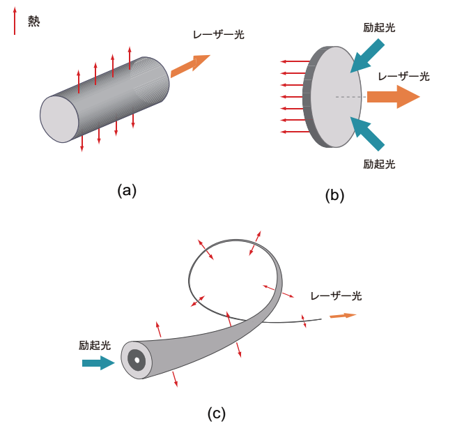
Fig.1.27 radiation properties for rod-type solid-state laser, disk laser, and fiber laser
0.3. Good beam quality
Laser light emitting from an optical fiber is easy to focus since the NA of fiber laser is relatively small. Therefore, the high-power density of output is realized, then high resolution processing is allowed. Furthermore, in implementing a fiber laser into a marking system, since small Galvano mirrors is available, a price reduction and a speeding up of the whole system is possible. In intergrating a singlemode fiber into the system constituion, the transverse mode can be almost perfectly unified.
0.4. Good lond-period stability
Because laser light is emitted from an optical fiber, the spatial fluctuation of laser beam is negligibly-small if the fiber is fixed. For all-fiber-type fiber laser where free-space optical setup is not included, thermal and mechanical effects caused by an attachment of grit and dust, and an surrounding environment are small since the all-fiber type fiber laser does not have any spatial optical device. Compared with CO2 laser, which is mostly used for laser processing applications, the fiber laser has both merits and demerits, but is superior in terms of short oscillation wavelengrth, good beam quality, and long focal depth. Therefore, the fiber laser can be used for processing an object put away from the focusing lens.
0.5. Wide gain width, high gain, high efficiency
Rare earth doped silica glass fiber, which is often used as a gain medium of fiber laser, is influenced by a complex crystalline field, and exhibits a broad level without micro-structure. Therefore, the rare earth doped silica glass fiber allows more wideband optical amplification than YAG crystal. In an optical fiber, even if a gain per unit length is small, a sufficient total gain is obained since the interaction length is long, Furthermore, because it is possible to confine the pumping light in the fiber, the highly efficient pumping is possible (optical-optical conversion efficiency:~70%, electric-optical conversion efficiency:~30%).
0.6. High-power
By serially or parallelly connecting modules, the amplification of output power is relatively easy. 50kW level super high-power CW fiber laser (transmission in fiber with the core diameter of 100µm ) has been already realized.
0.7 Long-distance propagation
Laser light emitted from the fiber laser can be efficiently coupled with a transmission fiber. By using the transmission fiber, it is possible to process an object put away from the laser body.
0.8 Nonlinear optical effect
In an optical fiber, because the core diameter is small and the interaction length is long, a nonlinear optical effect tends to be generated. Therefore, it is not appropriate for the high power pulsed operation, and may limit the characterisctics of laser. However, by using these properties, researches with a high novelty are eagerly performed.
1. Structure
Optical fiber is made of transmissive dielectric materials such as quartz glass (fused silica glass) and plastic. The optical fiber confines and transmits light by utilizing total internal reflection. The structure of typical optical fiber is double-layer: the first layer is core where light is confined and propagates, the other layer is clad which surrounds the core, as shown in Fig.2.1. In Fig.2.1, nair, n1, and n2 is the refractive index of air, core, and clad, respectively. The refractive index of core is a little bit higher than that of the clad, since an additive such as GeO2 and P2O5 is doped in the core. Therefore, light exhibits the total internal reflection at the boundary between the core and the clad repeatedly, and propagates in the fiber.
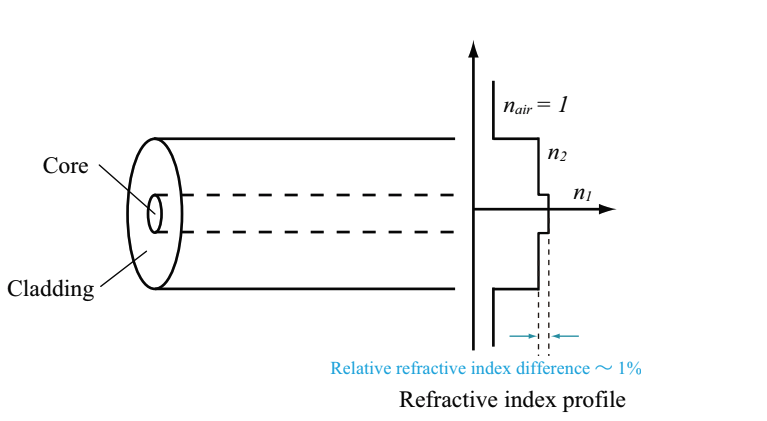
Fig.2.1 Structure of optical fiber
1.1. Critical angle & Relative refractive index difference
In optical fiber, the total internal reflection of light occurs when the propagation angle, θ, is smaller than the critical angle, θc (total reflection angle). Now we consider propagation light in optical fiber (see Fig.2.2). In Fig.2.2, n1, and n2 is the refractive index of the core, and the clad, respectively, and the critical angle, θc, is the incident angle, φ1, at the refration angle of φ2=90 (θ2=0).
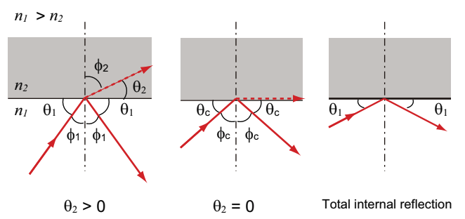
Fig.2.2 Schematic of critical angle and total reflection
Snell’s law is expressed as follows;
![]() (Eq. 2.1.1)
(Eq. 2.1.1)
therefore, the supplementary angle of the critical angle, θc, is defined by the following equation,
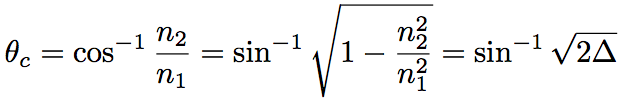 (Eq. 2.1.2)
where Δis relative refractive index difference, and is defined as follows.
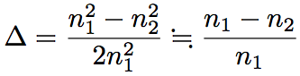 (Eq. 2.1.3)
Generally, the relative refractive index difference, Δ, is represented by percentage (%). A normal optical fiber has Δ ~ 4 %. In the optical fiber, since the refractive index difference is small, the critical angle is large.
1.2. Numerical aperature
Fig.2.3 shows a section of optical fiber. The maximal incident angle for the total internal reflection of light in the core is called as maximum acceptance angle, θmax. The maximum acceptance angle is represented by numerical aperture (NA).
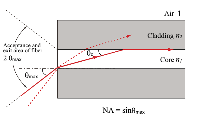
Fig.2.3 Numerical aperture of optical fiber
Provided that the surrounding of optical fiber is the air (nair=1), by combining Snell’s law at the fiber edge face and Eq.2.1.2, NA is obtained as follows.
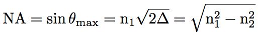 (Eq.2.1.4)
Eq.2.1.4 indicates that NA is controlled by changing the refractive index difference. For instance, provided n1=1.4675 and n2=1.4622, NA=0.125 is obtained. In order to efficiently introduce light in the optical fiber by using lens, it is usually better that NA of the lens is equal to or lower than NA of the optical fiber.
1.3. Coating
Optical fiber is coated by UV cure resin for its protection, when it is manufactured with delineation. UV cure resin used in the field of optelectronics is either of acrylate resin and epoxy resin. For the coating of optical fiber, the acrylate resin is used; Acrylate resin is the general term for methyl methacrylate polymer and its copolymer with acrylate.
Depending on whether optical fiber is coated or not, the optical fiber is named differently, optical fiber wire or optical fiber core wire. A typical structure of optical fiber is shown in Fig.2.4.
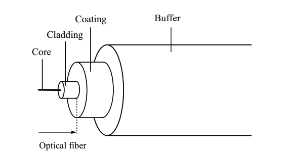
Fig.2.4 Optical fiber, optical fiber wire and optical fiber core wire
1.3.1. Optical fiber wire
In optical fiber wire (UV wire), only the UV cure resin is directly coated over the clad.
In a practical optical fiber wire, the coating is double-layer. The first coating over the clad is called as primary coating. The second coating on the primary coating is called as secondary coating. The role of primary, and secondary coating is the moderation of external stress, and resistance to the external stress, respectively. The double coatings of acrylate is called as dual acrylate resin coating (corting type: UV cured, dual acrylate).
For an optical fiber with the clad diameter of 125µm, provided that it has the primary and secondary coating with 30 µm thickness each, and a 5µm thickness coloring layer coated on the secondary coating for an identification of the fiber splicing point, its coating diameter is 250µm. This is 0.25mm optical fiber wire.
1.3.2. Core wire
The optical fiber wire does not have sufficient protection. For the core wire, polyamide resin (nylon) is coated over the wire.
The core wire is generally categorized into three types. In addition to 0.25mm optical fiber core wire (UV core wire), we have 0.9mm optical fiber core wire and the tape wire; a number of multi-core optical fiber are aligned in parallel by UV cure resin. Fig.2.5 shows those three types of optical fiber wire core.
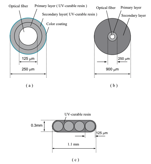
Fig.2.5 Various types of optical fiber core wires
(a) 0.25mm optical fiber core wire (UV core wire), (b)0.9mm optical fiber core wire, (c)Tape-type optical fiber core wire (4 Core Tape Core Wire)
Nylon core wire In nylon core wire, the UV cure resin or the silicon resin is employed for the primary coating, and the polyamide resin, nylon, is used for the secondary coating. For the sake of identification, the secondary coating is colored. The nylon core wire with 0.9mm outer diameter (the secondary coating diameter) is specially called as 0.9mm optical fiber core wire. Compared with the optical fiber wire, the nylon core wire is tough, and is superior in usability. The nylon core wire is often used for an optical fiber code and a LAN cable. The secondary coating like nylon is called as buffer. The buffer is categorized into two types, loose buffer and tight buffer. The tight buffer is directly attached on the optical fiber wire. The loose tube buffer utilizes plastic tube with a diameter several times larger than the fiber diameter.
Tape core wire In tape core wire, a number of 0.25mm optical fiber wire are aligned in parallel, and are coated in block by the UV cure resin. The tape core wire is used for composing a cable by placing fibers in a groove (tape slot structure). The tape core wires are typically double-core, quadruple-core, and octuple-core types.
2. Propagation property
If the incident angle of light is larger than the critical angle (θc), light can propagate with different optical paths in optical fiber (the number of optical paths is determined by the wavelength, quality, and property of propagating light). FIg.2.6 schematically represents light propagations in optical fiber at different incident angles. As is shown in Fig.2.6, in comparing the optical paths represented in the solid and dashed line, the optical path of dashed line is obviously longer, and the propagation time differs between these two light paths.
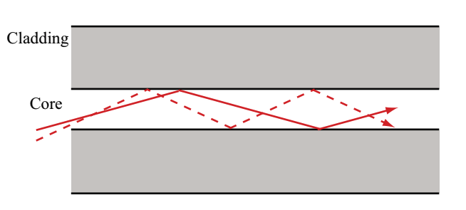
Fig.2.6 Mode of optical fiber
Each optical path for light propagation is called mode. The modes are discrete in optical fiber. This is because mode can not stably exist when the standing wave with nords at the core/clad boundary is not formed in the radical direction. Therefore, the mode in optical fiber is the transverse mode in a precise sense.
2.1. Fundamental and higher-order mode
The fundamental mode corresponds to the maximum incident angle to optical fiber (the mode closest to the fiber axis). The higher-order mode corresponds to the smaller incident angle compared with the fundamental mode. Provided that each mode is denoted as Nth-order mode, N is mode number. N represents the number of nodes in electric field distribution in the transverse direction. For the fundamental mode, N equals to 0. Fig.2.7 shows the field distributions of transverse electric (TE) mode corresponding to each mode number. The larger the mode number is, the larger the light leaking from the core to the clad is. Optical fiber usable for propagation of a number of modes is multimode optical fiber (MMF), optical fiber only for the fundamental mode propagation is single mode optical fiber (SMF). THe difference between SMF and MMF is yielded mainly from the core diameter difference. The relative refractive index difference of typical SMF is ca. 0.3%, and the typical core diameter is 2~10µm. The core doameter of MMF is in the range 7µm~3mm, and typically is 50, 62.5, 100, or 200µm. Particularly, in MMF used for optical communication, the core diameter is mostly either 50 or 62.5 µm.
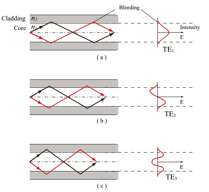
Fig.2.7 Mode number and field distributions of modes
(a) N=0, (b) N=1, (c) N=2
2.2. Mode dispersion
Mode dispersion indicates difference in the light propagation ttme between different modes. In case the mode dispersion is large, bit error is yielded. The mode dispersion does not occur in SMF since only the fundamental mode can exist., while the mode dispersion can cause an issue for MMF. The mode dispersion in MMF is minimized by arranging propagation delay time for all modes to be uniform (graded index (GI) type MMF).
2.3. Singlemode and multimode optical fiber
Single mode optical fiber (SMF) and two types of multimode optical fibers (MMF) are schematically shown in Fig.2.8. MMF is categorized into two types by the refractive index distribution in the core, step-index (SI) type optical fiber and GI type optical fiber.
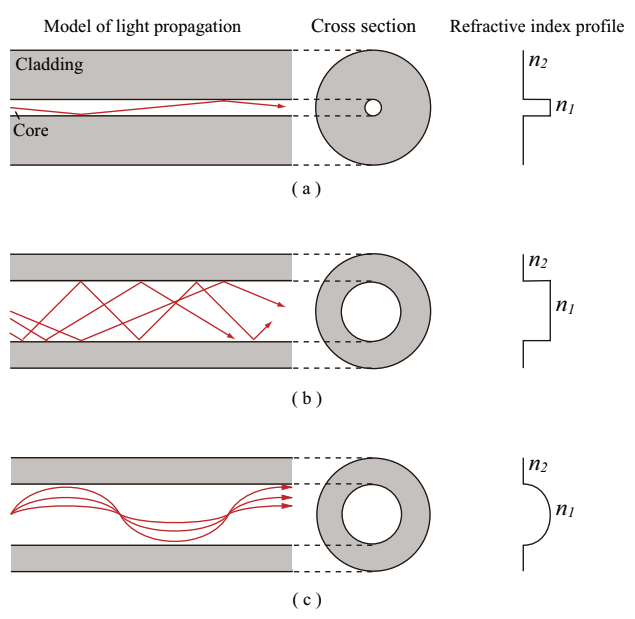
Fig.2.8 Light propagation and refractive index distributions of single mode optical fiber and two types of multimode optical fibers
(a) SI-SMF, (b) SI-MMF, (c) GI-MMF
2.3.1. Singlemode optical fiber (SMF)
As the core diameter decreases, the number of modes which can propagate in optical fiber decreases. For the core diameter smaller than a specific value, only the fundamental mode can exist. This kind of optical fiber is singlemode optical fiber (SMF). In SMF, it is theoretically proved that the light intensity distribution is close the Gaussian distribution.
Since the mode dispersion can not be zero even for GI-MMF, SMF is employed for the long-distance optical fiber communication. For a ultrashort pulsed light source, the SM propagation is the noly effective mode. This is because the MM propagating light is affected by the mode dispersion and mode noise.
2.3.2. SI type multimode optical fiber
In SI type multimode optical fiber (SI-MMF), the distribution of refractive index in the core is homogeneous. The refractive index steps down at the boundary from the core to the clad. Because the propagation angle is kept the same as the incident angle, the propagating distance in the core and the propagation time vary for each mode. Therefore, duration of the pulsed light incident to SI-MMF is elongated at the output edge after the light propagation in optical fiber. SI-MMF has a simple structure and is cheap, but its appplication is limited.
2.3.3. GI type multimode optical fiber
In GI type multimode fiber (GI-MMF), the refractive index is the highest at the core center. The refractive index is lower near the clad. Because of this, lower-order modes exhibit the total internal reflection in the vicinity of core center, while higher-order modes do it near the outer clad. Therefore, higher-order modes propagate a long distance in the core. However, since the light velocityis inversly proportional to the refractive index (v=c/n), light propagates faster at the outer side in the core where the refractive index is lower. By optimizing the refractive index distribution, the mode dispersion is minimized.
The stardard of measure of GI-MMF is determined by the advisory of ITU-T. The fiber loss is 0.8[dB/km] for core/clad=50/125µm and the length of 1310nm. GI-MMF has a larger transmission loss than SMF, but is used for the short-distance information communication such as LAN, because the fiber connection with network devices is easy.
2.4 Normalized propagation constant and waveguide parameter
In this section, we explain the normalized propagation constant and the waveguide parameter, which are the parameters featuring the optical fiber.
2.4.1. Normalized propagation constant
Provided the refractive index of core (n1) and clad (n2), and the light propagation angle (θ), mode propagation constant, β, is expressed by the following equation,
![]() (Eq.2.2.1)
(Eq.2.2.1)
where ko=2π/λ is the propagation constant of plane wave in air. By considering the range of propagation anlge, θ<π/2 and θ<θc, the possible range of β is given as follows.
![]() (Eq.2.2.2)
(Eq.2.2.2)
Eq.2.2.2 indicates that the propagation constant of waveguide mode can be a value between light wavenumbers in the core and the clad. Although the electric field of waveguide mode is confined and propagated in the core, a part of light is leaked toward the clad. This is possibly why the propagation constant take a value between the propagation constant for the core and the clad. As a normalized parameter of the propagation constant, the normalized propagation constant, b, is defined as follows.
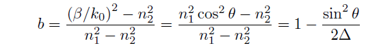 (Eq.2.2.3)
2.4.2. Waveguide parameter
The number of mode possibly existing in optical fiber is determined by the waveguide parameter (V parameter or normalized frequency). The V parameter is defined by the following equation,
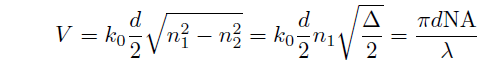 (Eq.2.2.4)
where d is the core diameter, NA=sinθmax is the core numerical aperture. The approximation curve for the singlemode dispersion is represented by using the normalized propagation constant, b, and the V parameter, as follows.
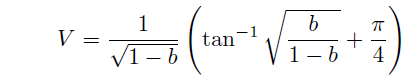 (Eq.2.2.5)
The normalized propagation constant and the V parameter for step-type optical fiber is shown as Fig.2.9. LPlm is the linearly polarized mode, and the detail is shown in Fig.2.10. Fig.2.9 is a pattern of LP mode obtaiend when the linearly polarized light is incident to optical fiber.
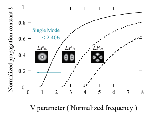
Fig.2.9 Dispersion curve of step-type optical fiber
At V=2.405, the cut-off occurs, for the propagation constant of LP11 mode equals to 0 (b=0). For V<2.405, only the LP01 mode is propagated (singlemode propagation). For V>2.405, a number of modes are propagated (multimode propagation). This and Eq.2.2.4 indicate that the V parameter increases for the relatively shorter wavelength, larger diameter, and larger refractive index difference, and that the number of propagation mode increases.
Fig.2.9 is also used for deriving the propagation constant, β.
By reading the norlamized propagation constant, b, at the V parameter given by Eq.2.2.4, and using Eq.2.2.3, the propagation constant, β, is calculated. The propagation constant, β, is used for calculations of the group velocity and its dispersion. For instance, let us consider an SMF with Δ=0.3, n2=1.460, and d=6.5µm, then, the refractive index, V parameter, normalized propagation constant, and propagation constant of the core at 1030 nm is calculated as n1=1.464, V=2.249, b=0.51, and β=8.9×10^6.
The LP mode is an approximated mode, and consists of vector modes (HE, EH, TE, TM). Table 2.1 summarizes the relationship between LP modes and the vector modes. Mode degeneration in the waveguide means the state where two or more modes have the same propagation constants with the diiferent electric field distributions. LP01, LP11, and LP21, shown in Fig.2.9, have the similar field distributions as (HE11 ), (TM01, TE01, HE21), and (HE11, HE31) have, respectively. Fig.2.10 represents the mode pattern for LPlm.
Table 2.1: Relationship between LP modes and the vector modes
| LP mode name | Vector mode name | Degeneracy |
| LP0m | HE1m | 2 |
| LP1m | TE0m, TM0m, HE2m | 4 |
| LPlm | HEl+1m, EHl-1m | 4 |
For step-type optical fiber, the relationship between the mode number and the V parameter is approximated as folliows.
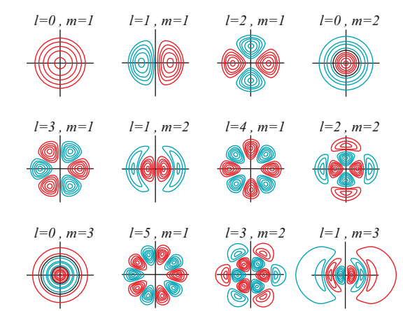
Fig.2.10 LPlm mode
 (Eq.2.2.6)
2.5. Mode field diameter and cut-off wavelength
2.5.1. Mode field diameter
In optical fiber, light propagates mainly through the core, but is partially leaked toward the clad. Especially for SMF, the diameter of the circular region for the light intensity of 1/e^2=0.135 of the core center light intensity is defined as mode field diameter (provided that the light intensity distribution in SMF is approximated by the Gaussian function). MFD is schematically explained in Fig.2.11. MFD, 2w, is usually a little bit larger than the core diameter, therefore is important as an effective parameter representing spatial volume of the light propagation. The idea of MFD is yielded since the core diameter and relative refractive index difference in SMF are small, then the boundary between core and clad is hard to be validly identified. For typical SMFs, MFD is in the range of 3~10µm.
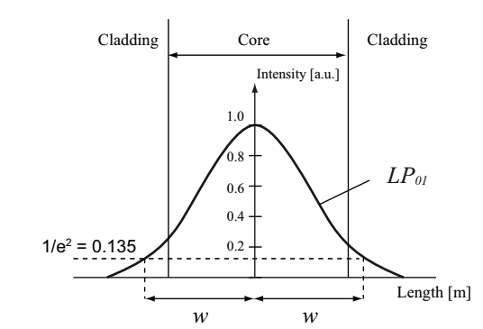
Fig.2.11 Schematic of mode field diameter
According to the ITU-T advisory, MFD is defined by the following equation,
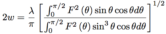 (Eq.2.2.7)
where F(θ) is the electric field distribution of far field pattern (FFP) and θ is the radiation angle to the propagation axis of optical fiber. MFD is also employed for evaluating the fiber splicing loss. The splice loss and MFD has the relationship shown in Eq.2.2.8.
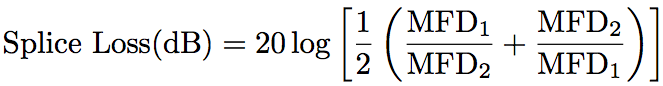 (Eq.2.2.8)
In Eq.2.2.8, MFD1 and MFD2 are MFD of a couple of fibers for splicing.
For SMF, the ratio of w to the core radius, a (w/a), is represented by the following function of V parameter.
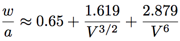 (Eq.2.2.9)
Eq.2.2.9 indicates that MFD is relatively smaller for the larger V parameter. Eq.2.2.9 can be used for the limited values of V parameter, 0.8~2.5.
2.5.2. Cut-off wavelength
Cut-off wavelength, λc, is defined in SMF as the shortest wavelength for which only the LP01 mode can propagate (singlemode propagation). Light with the wavelength shorter than λc exhibits LP11 mode propagation (multimode propagation). According to Eq.2.2.4, the cut-off wavelength for SMF is given by the following equation, that is, determined by the refractive index distribution and the core diameter.
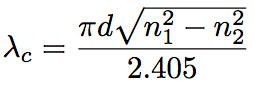 (Eq.2.2.10)
The cut-off wavelength can be directly measured by bending method or multimode excitation method.
3. Loss property
When light propagates in optical fiber, the optical power loss occurs. The power loss is an important parameter for characterizing a fiber. Provided that light at the optical power of P0 is incident to an optical fiber with a length of L, the optical power after propagation in the fiber, PT, is expressed by the following equation,
Eq.2.3.1
where α is the damping constant, representing loss in the optical fiber. The loss of optical fiber, α [dB/km], is generally given below.
Eq.2.3.2
Fig.2.12 shows the wavelength dependency of fiber loss for a typical quartz optical fiber. The fiber loss, αdB, takes the minimum value of ca. 0.2[dB/km] (damping constant α = 4.6 x 10^-7cm^-1) at the wavelength of ca. 1.55µm. The loss spectrum is determined by several factors. The primary factors are the absorption and the rayleigh scattering by the fiber material itself. The effect of Rayleigh scattering is relatively larger for a shorter wavelength of light. The Rayleigh scattering loss in the visible range is 1~10[dB/km], which is relatively smaller compared with a loss in other materials. Pure quartz glass has absorption bands only in the range longer than 2µm and in the UV range. However, when an even slight amount of impurity is added, the quartz glass has strong absorptions in the range of 0.5~2µm, which is transmissive for the pure quartz glass. In the following sections, the primary factors of optical fiber loss are explained with categorizing them into the loss attributable to material characteristics, the loss by impurity absorption, and the loss by structural imperfection.
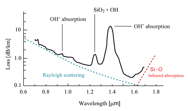
Fig.2.12 Wavelength dependency of fiber loss for a typical quartz optical fiber
3.1. Loss attributable to material characteristics
(1) IR absorption Light absorption of optical fiber in the IR range is attributable to the molecular vibration (lattice vibration) of SiO2 (IR absorption or molecular vibration absorption).
(2) UV absorption Light absorption of optical fiber in the UV range is due to the energy band transition of SiO2 (UV absorption or electron transition absorption).
(3) Rayleigh scattering The Rayleigh scattering is light scattering by a particle smaller than an incident light wavelength. A random density fluctuation, yielded in fused silica glass during the manufacturing process and fixed after, may cause the Rayleigh scattering. The density fluctuation yields the local fluctuation of refractive index, which scatters light in all directions. The loss by Rayleigh scattering is proportional to λ^-4, therefore is larger for light with relatively shorter wavelength. The scattering loss is inherent to a fiber, and determines the minimum value of fiber loss.
3.2. Loss by impurity absorption
(1) OH group molecular vibration OH ion exists in optical fiber. OH ion is impurity and causes loss in optical fiber. OH ion has an absorption by the fundamental vibration. The absorption peak is approximately at 2.73µm. The remarkable peak at 1.38µm and the small peak at 0.95µm shown in Fig.2.12 are due to the second-harmonic and third-harmonic overtones of OH absorption, respectively.
(2) Transition metal ion Light is absorped by transition metal ions, such as ions of Cu, Fe, and Cr. However, these transition metal ions are usually not mixed in optical fiber, since the fiber manufacturing process has been improved. Light absorption by transition metal ions is negligible.
3.3. Loss by structural imperfection
(1) Boundary loss If optical fiber had some irregularity at the core/clad boundary, light is emitted out of irregular parts. This emission loss is boundary loss.
(2) Microbending loss When unequal stress is applied to optical fiber in the radial direction, the fiber axis can be bent with a relatively small radius of curvature compared with the core diameter. This type of bending is called as microbending. The loss generated by the microbending is microbending loss.
(3) Bending loss Bending loss is yielded when optical fiber is bent with a large curvature, since the light does not exhibit the total internal reflection at the core/clad boundary, resulting in the partial emission of light out of the fiber. This is due to the fact that the incident angle to the boundary becomes smaller than the critical angle.
(4) Splice loss Splice loss is due to light leakage or misalignment of fiber axes at the splicing position. The cause of splice loss is mismatching of the core diameter or clad diameters between connected fibers. Recent developments in the fusion splicing technique enabled a low-loss splicing of a couple of different sorts of fibers.
4. Dispersion property
4.1. Phase velocity and group velocity
Light is electromagnetic wave. A propagation velocity of equivalent phase plane of electromagnetic wave is called as the phase velocity, vp. In a pulse propagation, an enegry transfer velocity of electromagnetic wave is called as group velocity, vg. For the electromagnetic (optical) pulse, the group velocity is a transfer velocity of envelope curve of a pulse.
Fig.2.13 explains the phase velocity, vp, and the group velocity, vg, for vp The group velocity, vg, depends on the frequency, and dvg/dw does not equal to 0. This frequency dependency is called as group velocity dispersion (GVD). An ultrashort pulse propagation is largely affected by GVD.
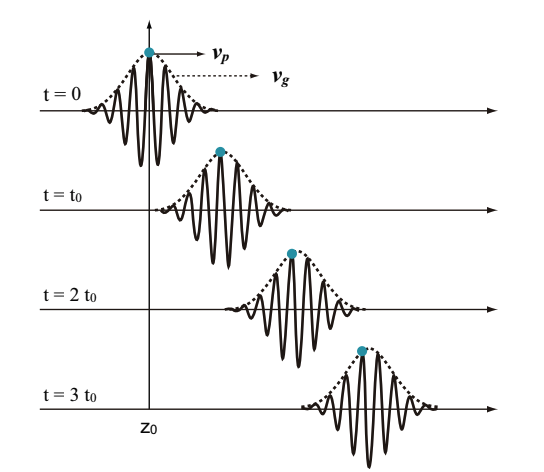
Fig.2.13 Phase velocity and group velocity in a pulse propagation (vp < vg)
4.2. Wavelength dispersion
The wavelength dispersion is a wavelength-dependent delay of llght propagation time. When an optical pulse is affected by the wavelength dispersion, the pulse duration is elongated. Fig.2.14 schematically explains the dispersion effect on optical pulse penetrating through a dispersive medium. Generally, “dispersion” means the wavelength dispersion, but not a mode dispersion and a polarized wave mode dispersion, although these are also optical fiber dispersions.
The wavelength dispersion is devided into a material dispersion due to a refractive index change in a materal and a waveguide dispersion due to a waveguide structure. The wavelength dispersion is the the sum of mateiral dispersion and waveguide dispersion. The material dispersion can not be controlled since it is inherent to a material itself (quartz glass, etc.). On the other hand, the waveguide dispersion is controlled by changing the core radius, the relative refractive index difference, and the the refractive index distribution.
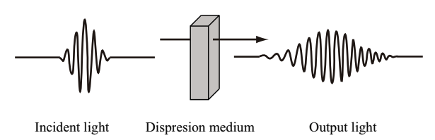
Fig.2.14 Schematic of dispersion
The wavelength dispersion is yielded by a frequency (wavelength) dependency of refractive index of an inductive medium. A propagation velocity of light in a medium with a refractive index of n(λ) is expressed as c/n(λ) where n is the light velocity in air. This means that the ilght velocity propagating in the medium is varied dependent on a wavelength of light.
According to the Sellmeier equation, derived by W.Sellmeier in 1871, a refractive index of medium, n(λ), is expressed by the following equation,
 (Eq.2.4.1)
where Ai is an intensity of light at a resonant frequency, νi, λi is given as λi=c/νi. Ai, λi, and m are constants depending on a material, and are estimated in experiments.
The Sellmeier equation can not give an accurate result in the vicinity of ν0 since it diverges at ν0. Excluding the frequency range, however, it approximates the wavelength dispesion with a good accuracy (for m=3, in the range of 365-2325nm, the precision of refractive index calculation is ±5×10^-6). The constants (Ai, λi) for various media can be obtained from “Handbook of Optical Constants of Solids” by E.D.Palik. For silica glass, at room temperature (18℃) and m=3, A1 = 0.6961663, A2 = 0.4079426, A3 = 0.8974794, λ1 = 0.0684043, λ2 = 0.1162414, and λ3 = 9.896161 are known, and the refractive index becomes lower as the wavelength becomes longer.
Eq.2.4.1 is rewritten as a function of frequency, n(ω), which is expressed by the following equation,
 (Eq.2.4.2)
where ωi equals to 2πc/λi.
4.3. Dispersion parameter
In order to show dispersion parameters of optical fiber, we perform the Taylor expansion of a mode propagation constant, β, around a center frequency, ω0. Then, the propagation constant is given as follows.
![]() (Eq.2.4.3)
(Eq.2.4.3)
 (Eq.2.4.4)
The parameter β1 and β2 are expressed as a function of refractive index, n, and its derivative.
 (Eq.2.4.5)(Eq.2.4.6)
In Eqs.2.4.5 and 2.4.6, ng is a group refractive index, and vg is a group velocity. β1=1/vg is a propagation delay time per unit length, and is called as a group delay time. β2 is GVD, which represents an elongation of pulse duration. In Fig.2.15, (a) shows the refractive index, n, and the group refractive index, ng, and (b) shows the the group velocity dispersion, β2, for bulk silica glass as a function of wavelength. λD in Fig.2.15 is the zero dispersion wavelength. For silica glass, the zero dispersion wavelength is approximately 1.27µm. The dispersion in Fig.2.15 is derived from the refractive index of slilica glass, and is called as a material dispersion. In a practical optical fiber, the core includes a slight amount of dopant such as GeO2 and P2O5, and the dispersion property depends on the conentration of dopant. For a material with the relatively larger refractive index (n), the absolute value of GVD is generally larger.
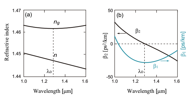
Fig.2.15 Dispersion characteristics of slilica glass
(a) Refractive index, n, and group refractive index, ng and (b) group velocity dispersion, β2 for slilica glass as a function of wavelength. λD is the zero dispersion. wavelength
In describing a dispersion of optical fiber, a dispersion parameter, D[ps/nm/km], is employed instead of GVD, β2[ps^2/km]. A relationship between the dispersion parameter, D, and the GVD, β2, is expressed as follows.
 (Eq.2.4.7)
The total dispersion of optical fiber is the sum of material dispersion and waveguide (structure) dispersion. The waveguide dispersion depends on the core radius and the refractive index difference between the core and the cald (Δ). By calculating the material dispersion and the waveguide dispersion from the references, and by summing them up, the total dispersion is obtained as shown in Fig.2.16. The zero dispersion wavelength, λD, for a typical optical fiber is 1.31µm. The zero dispersion wavelength of the material dispersion is redshifted bt the waveguide dispersion.
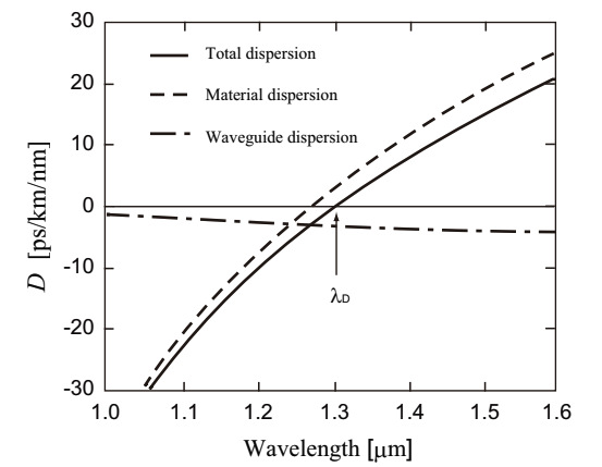
Fig.2.16 Total dispersion characteristics of slilica glass optical fiber
For λ<λD, we have D<0 (β2>0), and a fiber exhibits a normal dispersion. In the wavelength range of a normal dispersion, higher-frequency (shorter-wavelength) components in an optical pulse propagates relatively slowly compared with lower-frequency (longer-wavelength) components. On the other hand, the wavelength range of for λ>λD is callsed as a abnormal dispersion. The abnormal dispersion exhibits an opposite of the normal dispersion in terms of the characteristics of optical pulse propagation.
In the typical case, a dispersion indicates β2, the second order differential of β by ω. Higher-order dispersions indicate β3, the first order differential of β2 by ω, and the higher-order differential of β2 by ω. The higher-order dispersion must be considered for either a pulse in the vicinity to λ=λD or a relatively wideband pulse such as an ultrashort optical pulse with a duration of 100fs or shorter. In using a wideband optical pulse, the fundamental, the first-order, and the second-order items in Eq.2.4.3. are not enough for calculating a dispersion, therefore, higher-order dispersion must be considered.
Higher-order dispersions generally yield a distortion of wave shape. An optical pulse elongated by the second-order dispersion can be restored without much effort after the distorted pulse propagates through a dispersive material that cancels out the dispersion. In order to compensate the higher-order dispersions, a mode precise compensation is needed.
4.4. Dispersion control optical fibers
By utilizing the property that a waveguide dispersion depends on the parameters such as the core radius and the refractive index difference of core/clad, Δ, it is possible to control the zero dispersion wavelength, λD, and the dispersion slope. Fig.2.17 shows a dispersion characteristics for some of the controlled fibers: dispersion shifted fiber (DSF), nonzero dispersion shifted fiber (NZ-DSF), and dispersion flatted fiber (DFF). All of them is SMF.
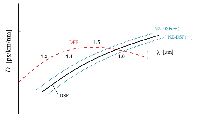
Fig.2.17 Dispersion characteristics for dispersion shifted fiber (DSF), nonzero dispersion shifted fiber (NZ-DSF), and dispersion flatted fiber (DFF)
(1) Dispersion shifted fiber For the zero dispersion wavelength, λD, to be shifted to ca. 1.55µm (a wavelength range for optical communication), the optical fiber loss is the minimum. This type of fiber is called as a Dispersion shifted fiber (DSF). DSF is appropriate for uses in long-distance transmission.
(2) Nonzero dispersion shifted fiber In a nonzero dispersion shifted fiber (NZ-DSF), the zero dispersion wavelength is slightly shifted from 1550nm band (usage wavelength range). Then, nonlinear optical phenomena such as four-wave mixing, self-phase modulation, and cross-phase modulation at 1550nm band is avoided.Therefore, NZ-DSF is useful for wavelength division multiplexing (WDM) using Erbium doped optical fiber amplification (EDFA) and for ultrafast long-distance transmission. In order to avoid a distortion of signal shape yielded by the wavelength dispersion, the value of wavelength dispersion is set to a relatively smaller value compared with a typical fiber.
(3) Dispersion flatted fiber Dispersion flatted fiber (DFF) exhibits the zero dispersion at 1.4µm and 1.6µm. In DDF, a complex profile of refractive index distribution controls the waveguide dispersion. DDF with a relatively small absolute value of dispersion is appropriate for transmission of ultrashort pulsed light, and can perform a wavelength conversion in the wide wavelength range including C-band range. With using higher nonlinearlity DFF, supercontinuum light with a super wideband spectrum is generated
(4) Reverse dispersion fiber For reverse dispersion fiber (RDF), the absolute values of wavelength dispersion and the dispersion slope are close to those of SMF, but the sign is opposite. Therefore, by combining RDF and SMF with the same fiber length, the wavelength dispersion and the dispersion slope are simultaneously compensated in the whole transmission path, and the zero dispersion is realized in the wide wavelength range (local wavelength dispersion is not zero). Thus, an optical fiber has both positive and negative areas of the wavelength dispersion in the direction of light propagation, and the integrated wavelength dispersion is decreased in the whole transmision path, although the local wavelength dispersion is not zero. This type of optical fiber is called as dispersion management fiber (DMF). DMF is commercially available. Since RDF has a higher nonlinearlity than SMF, RDF is arranged at the output side of transmission path in DMF.
4.5. Dispersion measurement method
A number of systems for wavelength dispersion measurement are produced by various manufacturers and are commerically available. The measurement methods are phase method, differential phase shift method, pulse method, interferometry method, and so on. In measuring the dispersion with these methods, it it nice to derive the wavelength difference by a differentiation after approximating the group delay with polynomial equation, called as the Sellmeier equation. Depending on a sort of optical fiber, an approximation formula used, and the number of measured wavelengths minimally required for the approximation are varied. In the following, for reference, an approximation formula, and equations for deriving a dispersion parameter, D(λ)=dτ(λ)/dλ, a zero dispersion wavelength, λD, and a dispersion slope, sD, for some Corning optical fibers are summrized. τ(λ) is a decay time for 1km propagation and has a unit of [ps/km]. Therefore, τ(λ) indicates an inverse of group velocity dispersion, vg, and is equivalent to β1.
(1) Normal singlemode fiber
(e.g.Corning SMF-28, SMF-28e)
 (Eq.2.4.8)(Eq.2.4.9)
(2) Dispersion shifted singlemode fiber
(e.g.Corning SMF/DS, SMF-LS)
 (Eq.2.4.10)(Eq.2.4.11)
(3) Other types of dispersion shifted singlemode fiber
(e.g.Corning LEAF, MetroCor)
 (Eq.2.4.12)(Eq.2.4.13)
In a dispersion measurement, the pulse intensity in optical fiber needs to be low in order to avoid nonlinear optical effects. The phase method, the differential phase shift method, the pulse method, and the interferometry method are briefly explain in the following texts. Each measurement method has a good or bad. It is better to select proper one out of the methods depending on a measuring objective.
Phase method and differential phase shift method
The phase method utilizes a number of light source emitting different wavelengths. Then, light with different wavelengths is input into a measured optical fiber, and differences in arrival time of signal light among each wavelength determine a value of wavelength dispersion. Concretely, when light with a certain wavelength is modulated by a constant frequency, the phase difference between input and output is read and recorded. By repeating this procedure with the number of wavelengths required for approximation, the Sellmeier equation is completed. Additionally, by measuring delay time, β1, depending on a wavelength and differentiating β1 with respect to ω, a value of β2 is obtained.
A similar measurement method is the differential phase shift method, in which a value of wavelength dispersion is directly measured provided that D(λ) is linear. As a light source, a group of light source with a small wavelength difference is employed. The Sellmeier equation is not used for the differential phase shift method.
Pulse method
In the pulse method, a group delay time for each wavelength in the time domain is directly measured. The approximation equation for wavelength dispersion is completed by a difference in arrival time among optical pulses with different wavelengths. A general configuration of pulse method is shown in Fig.2.18. The pulse method requires a knowledge on the delay in the testing device, and also requires an accurate calibration of device for a precise measurement. Since the pulse methods is utilizable only when pulses with different wavelengths simply propagate in a measured fiber, it has a merit of plain measurement. However, in measuring the delay time directly, a long optical fiber is necessary since a large delay time is required.
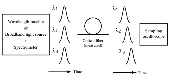
Fig.2.18 Configuration of dispersion measurement method for optical fiber(pulse method)
Interferometry method
The interferometry method utilizes a coherent light source (a wideband light source such as a supercontinuum light source). A Mach-Zehnder interferometer, which is composed of reference light path and a measurement light path including a measured fiber, is used for measuring an interferometric pattern of output, and for measuring a delay time at each wavelength. Fig.2.19 schamtically shows a typical configuration of interferometry method.
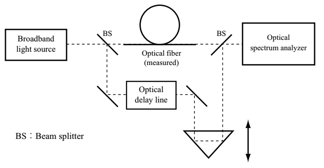
Fig.2.19 Configuration of dispersion measurement method for optical fiber(interferometry method)
① After splitting a broadband light into a couple of beams by a beam splitter, the one propagates through a measured optical fiber, the other propagates in a reference optical path.
② In a reference light path, an optical delay line is arranged since the interference of beams requires a matching of propagation time difference. Generally, an optical fiber with a well-known dispersion property is employed as an optical delay line, or a spatial delay plays a role of an optical delay line. A broadband light is affected by a wavelength dispersion in propagating through a measured optical fiber, and is delayed at an interference region depending on a wavelength. Therefore, the delayed broadband light temporally overlap with light having propagated through the reference path. At a specific wavelength, the phases are matched.
③ By measuring interference spectra with an optical spectrum analyzer with changing a length of reference optical path by a corner reflector, then measuring changes in the peak wavelength of interference, a relative delay difference at each wavelength is obtained,
④ In case an optical fiber is used as the optical delay line, obtained data contains a difference in a propagation delay for both the measuring path and the reference path. Therefore, the data needs to be calibrated after measurements.
The interference method utilizes, as it is named, an interference, and can precisely measure a relatively small change in the dispersion. The interference method is appropariate for uses in measuring a short-length fiber. However, in case an optical fiber is used as the optical delay line, an optical fiber with a dispersion equivalent to, or larger than, a duspersion of measured fiber is not available. The interference method requires a relatively precise operation in time compared with the pulse method.
5. Nonlinear property
5.1. Nonlinear optical effect
Silica optical fiber originally has a low nonlinearity. However, since laser light is confined in a narrow space (10µm or less in diameter) of optical fiber, the power density of electromagnetic field is high. Additionally, because an interaction length for a material and light is long, a variety of nolinear interactions are exhibited. In case an electronic field intensty is so high, the dielectric polarizability, P, is not proportional to the electric field, E, then, the higher-order components of polarizablity become nonnegligible (see the following equation).
 (Eq.2.5.1)
εo is a dielectric constant in the vacuum. χ are linear susceptibilities. The higher-order polarization is a nonlinear polarization.
(1) Second-order susceptibility The second-order susceptibility, χ^2, is related to second-order nonlinear optical effects such as second-harmonic generation and sum-frequency generation. in an optical fiber, however, since its molecular structure is symmetric, second-order nonlinear optical effects are generally not exihibited. Nonlinear optical effects in an optical fiber are caused by the third-order susceptibility, χ^3.
(2) Third-order susceptibility The third-order susceptibility, χ^3, is related to phenomena such as third-harmonic generation, four-wave mixing, nonlinear refractive index change, and nonlinear scattering. Among these phenomena, the third-harmonic generation and the four-wave mixing are generated only when the phase-matching condition is satisfied. Therefore, the most of nonlinear optical effects which occur in an optical fiber are the nonlinear refractive index change and the nonlinear scattering.
Phenomena yielded by the nonlinear refractive index change can be self phase modulation (SPM), a phase shift of light in an optical fiber, which is induced by its own, cross phase modulation (XPM) induced by different rays of light, and so on.
The nonlinear scattering occurs in case a light intensty exceeds a certain threshold in glass, and is due to an interaction between light and sound wave (phonon) generating in glass. When highly intense light travels in an optical fiber, molecular vibrations of SiO2 occur and the generated phonon propagates. The vibration of diatomic molecule such as SiO2 is categorized by a relative direction of diatomic vibration; one is the same direction, and the other is an opposite direction. The former is acoustic vibration (acoustic phonon), while the latter is optical oscillation (optical phonon). Scattering by the acoustic phonon is stmulated Brillouin scattering (SBS). Scattering by the optical oscillation is stimulated Raman scattering (SRS). These kinds of nonlinear scattering are featured by a wavelength shift in the scattering light, compared with a linear scattering. Stokes light (scattering light) is redshifted relatively to1064nm, a wavelength of incident light, by ca. 0.06nm for SBS and ca. 52nm for SRS. In a femtosecond laser osciilator with a high peak intensity, SRS is remarkable, while SBS is remarkable for a nanosecond laser amplifier with a high average power.
The principle nonlinear optical effects in an optical fiber is briefly summarized in table 2.2.
Table 2.2: Principle nonlinear optical effects in an optical fiber
| Item | Brief description |
| Self phase modulation (SPM) |
Phase shifted by own light intensity |
| Cross phase modulation (XPM) |
Phase shifted by light intensity of another light |
| Four-wave mixing (FWM) |
New wavelengths of light are generated when light of two or more different wavelengths is injected into the fiber |
| Stimulated Raman scattering (SRS) |
Optical vibration shifts the wavelength of scattered light to longer wavelengths (approx. 52nm @1064nm) |
| Stmulated Brillouin scattering (SBS) |
Acoustic vibration shifts the wavelength of scattered light to the longer wavelength side (approx. 0.06nm @1064nm) |
5.2. Nonlinear refraction
Nonlinear refraction is a light intensity dependency of refractive index attributable to the third-order susceptibility, χ^3, and is also called as the optical Kerr effect. The refractive index change due to the optical Kerr effect is expressed as a function of time, n(t), and is proportional to a light intensity, |E(t)|^2.
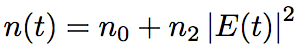 (Eq.2.5.2)
n0 is a linear (small-signal) refractive index of medium. n2 is a nonlinear refractive index coefficient, n2=3.18×10^-20m^2/W for silica glass optical fiber.
5.2.1. Nonlinear coefficient and effective core cross-section
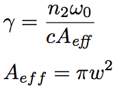
Nonlinear optical effect is characterized by nonlinear coefficient, γ. Since the nonlinear coefficient, γ, is related to the nonlinear refractive index coefficient, n2, and the confinement of light in an optical fiber, it is useful for evaluating the nonlinearity. The nonlinear coefficient, γ, is given as follows.
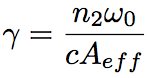 (Eq.2.5.3)
Aeff is an effective core cross-section, which represents a degree of optical confinement in an optical fiber. Provided a mode distribution in an optical fiber in the cross-sectional direction, F(x,y), Aff is expressed by the following equation.
 (Eq.2.5.4)
For SMF, since a mode distribution in an optical fiber is approximated by a Gaussian function, the effective core cross-section, Aeff, is simply given by the following equation.
 (Eq.2.5.5)
The nonlinear coefficient, γ, can be measured by using self phase modulation, cross phase modulation, four-wave mixing, optical soliton, and so on.
5.2.2. Self phase modulation
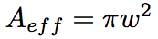
Self phase modulation (SPM) is induced by the optical Kerr effect. SPM is a phenomenon that a optical phase is shifted (light is modulated in phase) by its own, which induces a refractive index change when light is propagated in an optical fiber. Fig.2.20 schmatically explains SPM. Fig.2.20(a) indicates the intensity of light propagating in the optical fiber, and (b) indicates a refractive index change by the propagation light in the optical fiber. At the pulse center, since the light intensity is relatively high, the refractive index is larger compared with both edges.
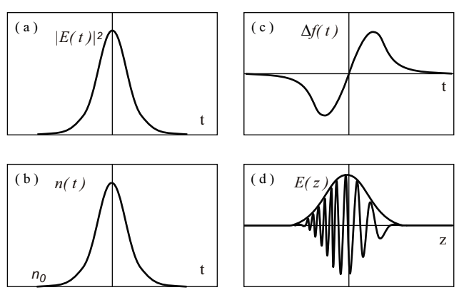
Fig.2.20 Frequency chirp by self phase modulation
In the case that an optical pulse travels a slight distance, Δz, in an optical fiber with a refractive index, n, the phase of electric field is temporally delayed at the exiting side compated with the input side. The phase shift at the exiting side is expressed by the following equation,
![]() Eq.2.5.6
Eq.2.5.6
where k is a wavenumber in the vacuum. With considering Eq.2.5.2, the phase shift, Δφ(t), is represented as follows.
 Eq.2.5.7
Eq.2.5.7 indicates that the phase shift is modulated depending on the pulse intensity, |E(t)|^2.
A shift of instantaneous angular frequency, Δω(t), by SPF is a rate of temporal change in the phase shift, Δφ(t), then an instantaneous frequency shift, Δf(t), is expressed as follows (see also Fig.2.20(c)).
 Eq.2.5.8
The instantaneous frequency shift due to SPM decreases in proportion to the first order temporal differentiation of pulse intensity phase, |E(t)|^2. For n2>0, the frequency is lower at the front edge of pulse, while it is higher at the rear edge (see Fig.2.20(d)).
Thus, SPM can be used for generating other frequency components and elongating the pulse duration. As light energy becomes higher, the pulse duration becomes longer. The frequency change between the front edge and the rear edge of pulse is called as chirp. Chirp for the rear edge to be higher is called as positive chirp, while chirp for the rear edge to be lower is called as negative chirp,
5.2.3. Four-wave mixing
Four-wave mixing (FWM) is a sort of optical parametric oscillation, and is generated when light with two or more different wavelengths are introduced into an optical fiber. When light with three different wavelengths are input into an optical fiber, light with a different wavelength from all the others is generated. The generated light is called as idler light. FWM affects SRS in any medium, and the effects on SRS in an optical fiber has been studied in detail.
FMW occurs when photons of a single or more waves disappear and other photons with different frequency is generated. The generated photons obey the conservation laws of energy and momentum of a parametric interaction.
Here, we consider that we have four different light waves at frequencies of ωp1, ωp2, ωprobe, and ωidler, respectively. FMW is either of ① different three photons are energetically converted to single photon with ωidler = ωp1+ωp2+ωprobe ② different two photons with frequencies of ωp1 and ωp2, respectively, disappear and at the same time, different two photons with frequencies of ωprobe and ωidler are generated based on a relationship of ωidler = ωp1+ωp2+ωprobe.
・Case ① It is difficult to efficiently satisfy a phase-matching condition of FWM. However, for ωp1 = ωp2+ωprobe, third-harmonic generation occurs, and for ωp1 = ωp2≠ωprobe, a frequency conversion of ωidler = 2ωp1+ωprobe occurs.
・Case ② If the condition of ωp1 = ωp2 is satisfied, a condition for FWM is relatively easy to be satifsfied. Degenerated four-wave mixing (DFWM), in which a part of light waves are degenerated, is mostly studied with optical fibers. DFWM is physically similar to SRS, that is, a couple of photons emitting from intense pumping light (ωp = ωp1 = ωp2) is converted to probe light (ωprobe) and idler light (ωidler = 2ωp – ωprobe).
Fig.2.21 explains FWM with a schematic figure. (a) shows the case that two waves are used as pumping light, and (b) shows the case that single wave is used as pumping light (DFWM).
Fig.2.21 Schematic of four-wave mixing in the frequency range
The case that (a) two waves are used as pumping light, (b) single wave is used as pumping light (DFWM)
In wavelength division multiplexing (WDM), FWM generated with multiplexed signal decreases a quality of transmission. When signal with a variety of wavelengths is arranged with a constant interval, noise by FWM is generated over used wavelengths and induces a signal distortion. As a zero dispersion is close to the wavelengths, an generation efficiency of noise by FWM (wavelength channel crosstalk) is high. Therefore, an use of dispersion shifted fiber (DSF) particularly causes an issue of noise generation in C-band range. In WDM system, an use of nonzero dispersion shifted fiber (NZ=DSF), which does not require zero wavelength dispersion in the vicinity to an usable wavelength range, is effective for avoiding the FWM noise. Although FWM causes an issue in WDM transmission, since it can generate light with a certain wavelength out of light with different wavelengths, it is eagerly studied for a wavelength conversion device.
Compared with a variety of wavelength conversion methods, which have been suggested, FWM is advantageous of the conversion speed and the conversion simultaneity over a certain wavelength range. The following four treatments are further effective for increasing the FWM efficiency and broadening FWM in the wavelength range: (1) matching a wavelength of pumping light and a zero dispersion wavelength of optical fiber, (2) lowering a shift of wavelength dispersion in the axial direction of optical fiber, (3) matching polarization directions betwen pumping light and probe light, (4) Shortening a fiber length by using a highly nonlinear optical fiber (fiber length ≤ coherent length).
5.3. Nonlinear scattering
Third-order nonlinear optical effects (χ^3) such as third-harmonic generation and four-wave mixing occur via light-induced modulations of medium parameters such as a refractive index. Since any energy trasfer does not occur between light and a nonlinear medium, a third-order nolinear optical effect is called as parametric process (featured by the fact that quantum mechanical initial and end states are the same). On the other hand, SRS and SBS are nonparametric processes where a part of light energy is transferred to a nonlinear medium.
5.3.1. SRS: Stimulated Raman Scattering
When intense pumping light is incident to a nonlinear medium with exceeding a certain threshold (Raman threshold), Stokes light, a lower-frequency light, is rapidly amplified, then the most of energy of pumping light is transferred to the energy of Stokes light. This phenomenon is SRS. A frequency difference between the pumping and Stokes light us called as Raman shift or Stokes shift. SRS is an important nonlinear process for functioning a Raman amplifier and a fiber Raman laser. Raman shift for 1064nm wavelength is approximately 52nm, while a shift for the maximum Raman gain with 1064nm pumping light is 116nm,
In a quantum mechanical description, Raman scattering is cconsidered as a lower-frequency convesion process, in which a pumping photon is converted to a lower-frequeny photon and a phonon of molecular vibrational mode. Although a phonon coupling with a pumping photon can generate a higher-frequency photon, this higher-frequency conversion barely occurs in practice since a phonon with proper energy and momentum does not exist a lot. This higher-frequency light is called as anti-Stokes scattering, which has a frequency of ωa = ωp + Ω, while Stokes light has a frequency of ωs = ωp – Ω
Fig.2.22 schematically represents mechanisms of Stoke scattering and anti-Stokes scattering. Stokes-scattering occurs when a molecule transferred to an intermediate state by incident light is relaxed to a vibrational exictated state, while anti-Stokes scattering occurs when a thermally excited molecule is transferred to an intermediate state by incident light, then relaxed to a ground state.
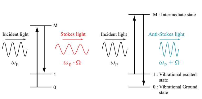
Fig.2.22 Mechanisms of Stoke scattering and anti-Stokes scattering
When anti-Stokes scatterig occurs, 2ωp=ωa+ωs is obtained from ωs=ωp-Ω and ωa=ωp+Ω. Therefore, when a momentum is conserved, an FWM process where a couple of pumping photons disapprear and a single Stokes and anti-Stokes scattering photons are yielded. This momentum conservation condition is a phase-matching condition, Δk=2kp-ka-kx=0, for FWM. If the phase-matching condition is not satisfied, FWM does not occur.
(1) Raman gain spectrum Raman gain strongly depends on an polarization interaction between pumping light and signal light. Let us consider a case that excitation light is linearly polarized. When probe light is linearly polarized in parallel to the excitation light, Raman gain (parallel Raman gain), g||, is large. On the other hand, when probe light is linearly polarized in perpendicular to the excitation light, Raman gain (perpendicular Raman gain), g⊥, is small. Fig.2.23 represents a parallel Raman gain, g||, of silica optical fiber as a function of a frequency shift. The vertical axis is shown with normalized by the maximum value of Raman gain.
Fig.2.23 incidates that Raman gain, gR, has a peak at around 13THz with a broad expansion to 40THz. This is because frequency distributions of molecular vibration in amorphous material such as quartz glass are continuously overlapped. This characteristics has an optical fiber functioning as a wideband amplifier. Since the gain specturm is broad, a response time is in the femtosecond range. However, in case SRS is induced by a pumping pulse with a duration of 100ps or shorter, effects of GVD, mismatch of group velocity, self phase modeulation, and cross phase modulation need to be considered.
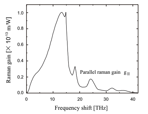
Fig.2.23 Raman gain spectrum of silica optical fiber
(2) SRS threshold SRS is either forward SRS or backward SRS. In case that pumping power is increased, the forward SRS first experiences its threshold, and the backward SRS is generally not observed in an optical fiber. The forward SRS threshold (critical pumping power), PthSRS, is expressed by the following equation,
 (Eq.2.5.9)
where Aeff is an effective core cross-section, leff is an effective interaction length, and α is a fiber loss at a wavelength of pumping light. For the backward SRS, 16 in the right side of Eq.2.5.9 is changed to 20.
(3) Stokes light process When only the pumping light is incident to an optical fiber, spontaneous Raman scattering is first generated, then is amplified with its propagation. Since spontaneous Raman scattering contributes to all the range of Raman gain spectrum, components in the whole frequency range is amplified, but light with the frequency for maximum gR (13.2THz or 440cm-1 for pure quartz) is maximally amplified. If pumping power exceeds the Raman threshold, light with this frequency is nearly eponentially amplified (Stokes light). Then, if Stokes light is sufficiently intense, it can induce higher-order Stokes light. The number of higher-order Stokes components is determined the incident pumping power. Intense pumping power can continuously induce N times Raman scattering, then enabling a wavelength conversion of N x 440cm-1.
When pumping light and weak signal light are simultaneously introduced to an optical fiber, a signal light with a wavelength in the range of Raman gain spectrum of pumpin light is amlified. This is a fundamental mechanism of fiber Raman amplifier. In case CW or nanosecond pulse is used for he pumping, SBS threshold is lower than SRS threshold, then SBS becomes dominant. In case a femtosecond pulse with a high peak intensity is used as pumping light, SRS is remarkable.
5.3.2. SBS:Stimulated Brillouin Scattering
Stimulated Brilloin scattering (SBS) is described as a nonlinear interaction among incident light, Stokes light, and accoustic phonon. Fig.2.24(a) and (b) show schematic mechanisms of SBS for input of short pulse laser with intensity close to SBS threshold and long pulse laser satisfying the SBS condition, respectively.
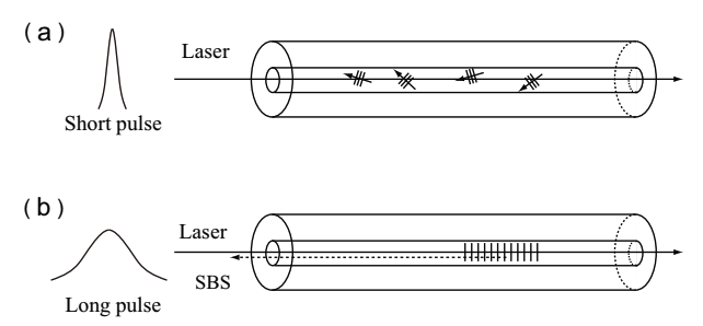
Fig.2.24 The case that (a) SBS for input of short pulse laser with intensity close to SBS threshold and (b) long pulse laser satisfying the SBS condition
In case intense coherent light is input to a optical fiber, an accoustic phonon is generated and a periodic modulation of reftractive index (working as grating) is yielded as shown in Fig.2.24(b). The incident light exhibits the Bragg reflection by the grating and is returned. Since the grating moves with a soudn velocity, vA, backward scattering of incident light (Stokes light) is blueshifted by the Doppler shift. Because of the stimulated emission effect of scattering light, SBS becomes an intense coherent light. A frequency shift is determined by a nonlinear medium, and is shows as a wavelength difference between incident light and Stokes light. This is expressed by the following equation,
 (Eq.2.5.10)
where vi is a frequency of incident light, vs is a Stoke frequency, n is a fiber refractive index, and λi is a wavelength of incident light. For silica glass, the sound velocity is VA=5/96[km/s] and the refractive index is n=1.45. Therefore, at λi=1064nm, vB is 16/2GHz.
SBS is also a kind of nonlinear scattering, the same as SRS. But the Stokes light if SBS propagates backward, while the Stokes light of SRS propagates in forward (θ=0) and backward (θ=π) directions. The Stokes shift of SBS is three digits smaller than the Stokes shift of SRS (~10GHz).
(1) Brillouin gain coefficient The amplification of Stokes light is featured by the Brillouin gain coefficient, gB(v), which has a maximum value at v=vB. The Brillouin gain width, ΔvB, is obtained by the following equation.
 (Eq.2.5.11)
The Brillouin gain is a function of accuostic relaxation time, in other words, phonon lifetime, τB. Provided that an accoustic wave is decayed with exp(-t/τB), the brillouin gain is expressed by a Lorentzian spectrum,
 (Eq.2.5.12)
where we have the following equation.
 (Eq.2.5.13)
p12 is a transverse optical elastic coefficient, ρ is a mateiral,density, and λi is a wavelength of incident light. The Brillouin gain was first measured at bulk quartz in 1950. The Brillouin gain of silica optical fiber is so different from that of the bulk quartz. This is because the core of optical fiber is doped with Ge and so on to increase its refractive index. The decrease in Brillouin gain is inversely proportional to the increase in Ge concentration. The Brillouin gain of silica optical fiber is gB=1.2 x 10^-11[m/W] for λ = 1.0 μm, τB = 2.3ns, ΔνB = 138.4 MHz, p12 = 0.286, and ρ = 2.202×10³ [kg/m3].
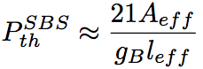
SBS threshold A threshold of incident pumping power for SBS depends on a spectral width and a pulse duration. SBS barely occurs with a short pulse duration (<1ns), while SBS occurs in using laser with a narrow spectral width such as a CW and a longer pulse (>100ns) laser. SBS threshold in an optical fiber becomes relatively small as a fiber length is long, a fiber core diameter is small, and a fiber loss is low. Typically, in a low-loss (<0.2[dB/km]) SMF, SBS threshold is as low as several mW for a fiber length of ca. 20km. A pumping power threshold for SBS is expressed by the following equation,
 (Eq.2.5.14)
where gB is a maximum value of Brillouin gain given by Eq.2.5.13, Aeff is an effective core cross-section, and leff is an effective interaction length. gB is determined by an accurate spectral width of Brillouin gain, and is approximated to be 21. This equation includes a lot of uncertainties, but is useful for guessing a SBS threshold.
A transient response of SBS depends on an indicent width and phonon lifetime. For Aeff ≈ 7.9 × 10⁻¹¹m^2 (core diameter of 10μm), gB = 10 × 10^−11 [m/W], and leff = 5 m, PthSBS is lower than 4W. A steady-state operation of SBS process requires 10~20 times longer duration for an incident pulse compared with accoustic relaxation time of SBS medium. For silica glass, since the accoustic relaxation time is 2.3 ns, an incident pulse with a duration of 23~46ns is required. For longer duration pulses, SBS thresholds will be almost constant.
5.4. Optical soliton effect
Optical soliton is generated when a pulse expansion by a dispersion effect in the abnormal dispersion range and a pulse compression by SPM are balanced in an optical fiber. Soliton is named from solitary wave. A wave shape of soliton is maintained even when the soliton propagates for a long distance. The soliton is not affected by its collision with each other. The optical soliton was discovered in 1973 by Akira Hasegawa, AT & T Bell laboratory, USA.
Assuming that an optical fiber is in the normal dispersion range at a wavelength of incident optical pulse, a front component with a long wavelength propagates faster, while a rear component with a short wavelength propagates slower, then the pulse is expanded (wavelength dispersion). In the normal dispersion range, SPM also contributes to the pulse expansion.
In the abnormal dispersion range, a front component of pulse propagates slower, while a rear component of pulse propagates faster. Therefore, in the abnormal dispersion range, a pulse duration is expanded by the wavelength dispersion, but is compressed by SPM. When the pulse expansion and cimpression are balanced, an optical pulse in fiber propagates with maintaining the wave shape. This pulse is the optical soliton, and this phenomenon is called as the optical soliton effect. Fig.2.25 shows the mechanism of optical soliton generation.
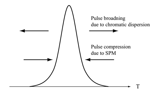
Fig.2.25 The mechanism of optical soliton generation
Optical soliton and nonlinear Schroedinger equation
An optical soliton is expressed by solving a nonlinear schroedinger equation. Provided an envelope function of optical pulse, A(z,T), an optcal soliton is expressed by the following equation,
 (Eq.2.5.15)
where P0 is a peak power of optical pulse, and To is a pulse duration. T0 is related to an FMHM of light intensity, TFMHM, at TFMHM=1.763T0. The peak power, P0, satisfies the equation shown below,
 (Eq.2.5.16)
where γ is a nonlinear coefficient. For a pulse input with a higher peak power than obtained by Eq.2.5.15, higher-order soliton solutions exist. A soliton order, N, which determines an order of higher-order solitons, is given as follows.
 (Eq.2.5.17)
For generating an Nth-order soliton, a N^2 time higher peak power than required for a fundamental soliton generation is necessary. The pulse shape of higher-order soliton periodically changes when a soliton propagates in an optical fiber. The period of propagation is called as soliton period. A soliton is generated with a soliton period, z0, given by the following equation.
 (Eq.2.5.18)
Soliton order
Soliton order, N, is a parameter representing which dominantly affects an optical pulse, a nonlinear optical effect, or a dispersion effect.
(1) N<1 For N<1 (in practice, a soliton order at an input phase smaller than 0.5 is only possible), a dispersion affects a pulse. Therefore, an optical soliton is not formed and a pulse is temporally expanded with its propagation. (2) N=1 For N=1, an dispersion effect and a nonlinear optical effect are balanced. The first-order soliton pulse propagates with maintaining the shape both in time and frequency, and is called as a fundamental soliton. (3) N>1 A higher-order soliton at N>1 propagates in an optical fiber with changing its shape at a constant period. The most characteristic property of higher-order soliton is a pulse compression process necessarily yielded at the begining of cycle.This is because a pulse compression caused by SPM chirping is remarkable compared with a pulse expansion caused by a dispesion since a nonlinear optical effect affects a pulse at the begining of cycle. This process is called as a high-order pulse compression, and is applicable to an ultrashort pulse generation.
Since the higher-order soliton compresses a pulse depending on a soliton order, N, its compression factor is larger than for the normal dispersion fiber compression and the abnormal dispersion fiber compression. However, in the higher-order soliton compression, only the center of pulse is compressed, while the edges are not compressed, then the pulse shape is changed to an island shape. This island-shaped component is called as pedestal. The pedestal at the edges of pulse can not described by any function form (such as sech-type functions), and is larger than a function value that is decayed at a time delay (see Fig.2.26). The pedestal is yielded since the chirp induced in SPM is linear at a center of pulse and only the center part is compressed by the abnormal dispersion of optical fiber. The pedestal is larger for a larger soliton order, N.
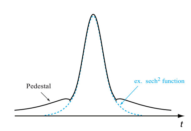
Fig.2.26 Schematic of pedestal
5.4.1. Soliton self frequency shift
SRS induces the phenomenon named soliton self frequency shift (SSFS) when combined with an optical soliton. For a fundamental soliton with a pulse duration shorter than 1ps, the spectral width is sufficiently large; A spectral width has the relationship of Fourier transform with a pulse duration. Then, SRS occurs in the pulse, and a shorter wavelength component amplifies a longer wavelength component; The energy of shorter wavelength component is continuously shifted to the longer wavelength component. Since this process lasts during a pulse propagation in an optical fiber, as a propagation length in the fiber is longer, the optical soliton is shifted to a longer wavelength region. This phenomenon is SSFS.
5.5. Numerical analysis
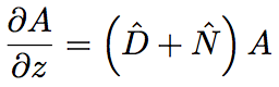
Numerical analysis of behaviour of optical pulse propagating in an optical fiber is important upon constructing a fiber laser system. In this section, we describe a nonlinear Schroedinger equation representing a behaviour of ultrashort pulse in an optical fiber and split step Fourier method, a numerical method for analyzing the Schroedinger equation.
5.5.1. Nonlinear Schroedinger equation
A propagation of optical wave in an optical fiber is represented by the Maxwell’s equations. Generally, rapidly varying components of electric field are igonored and a behaviour of optical pulse is approximated by a slowly varying envelope curve in order to simplify the calculation. In case a time system of group velocity of pulse (decay coordinate system) is utilized, a propagation equation for an envelope function of optical pulse, A(,T), is expressed as follows.

 (Eq.2.5.19)
γ is a nonlinear coefficient. This equation is called as nonlinear Schroedinger equation and is often used for a decription of ultrashort pulse propagation in an optical fiber. In the left side of Eq.2.5.19, the second term represents a fiber loss, and the third term represents an effect of wavelength dispersion including higher-order dispersions. The right side of Eq.2.5.19 represents nonlinear optical effects such as SPM, FWM, self-steeping, and SRS. R(t) is a Raman response function, and is contributed by both electronic and vibrational (for Raman) transitions. Fig.2.27 shows a delayed Raman response function, hR(t), calculated from the Raman gain spectrum in Fig.2.23 (an experimental result).
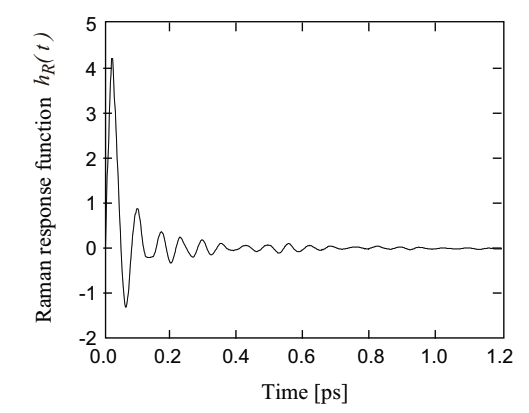
Fig.2.27 Raman gain response function
Assuming that an electronic transition occurs instantaneously, a Raman response function, R(t), is expressed by the following equation,
 (Eq.2.5.20)
where fR is a contribution ratio of delayed Raman response given by Ra(t)+Rb(t). Ra(t) and Rb(t) are Raman response functions corresponding to ga and gb shown in Fig.2.28, respectively. ga and gb are a couple of decomposed components of parallel Raman gain, g||. g⊥ is a perpendicular Raman gain.
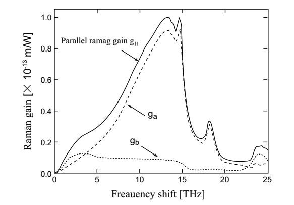
Fig.2.28 Parallel Raman gain spectrum
The Raman response function Ra(t) can be approximated by the following expressions,
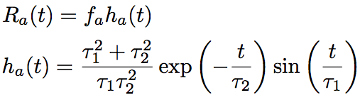 (Eq.2.5.21)(Eq.2.5.22)
where τ1 and τ2 are regulation parameters. τ1=12.2fs, τ2=32fs, and fs=0.75 are adopted since they are very close to a practical Raman gain spectrum. The Raman response function Rb(t) can be approximated by the following expressions.
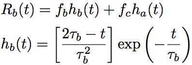 (Eq.2.5.23)(Eq.2.5.24)
Provided fb=0.21, fc=0.04, and τb=96fs, and fR=0.245, the Raman response function R(t) is properly approximated in the frequency range of 0~15THz.
Thus, Eq.2.5.19 includes higher-order dispersions and nonlinear optical effects, and accurately reproduces an effect of delayed Raman response. Therefore, by using Eq.2.5.19, it is possible to accurately analyze a temporal evolution of ultrashort pulse with a duration of 20~30fs. However, for a pulse shorter than10fs, since the slowly varying envelope approximation is broken down, Eq.2.5.19 is not usable. For this ultrashort pulse, the Maxwell’s equations must be directly solved by using numerical integral.
For a pulse with a duration with ca. 50fs or shorter, Eq.2.5.19 can be simplified as below.
 (Eq.2.5.25)
By applying the Taylor expansion to |A(z,t-t’)|^2 in Eq.2.5.19 and considering the zeroth- and first-order terms of t’, the following relationship is obtained.
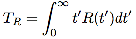 (Eq.2.5.26)
TR is associated with a slope of Raman gain spectrum, and is motly ~5fs. The first, second, and third terms of right side of Eq.2.5.25 represent self phase modulation, self steeping, and Raman effect, respectively.
5.5.2. Split step Fourier method
For the propagation equation, an analytical solution typically can not be obtained, since the nonlinear Schroedinger equation used as the propagation equation is a nonlinear partial differential equation. Therefore, a numerical analysis is employed for understandings of nonlinear optical effects yielded in an optical fiber. In the following paragraphs, we focus on split step Fourier method as a calculation method and explain a method to analyze behaviours of pulse in an optical fiber. Because the split step Fourier method employs an algorithm of fast Fourier transform (FFT), the analysis speed is faster than most of other analytical methods.
In order to explain the split step Fourier method, we use Eq.2.5.25. First of all, we deform Eq.2.5.25 into the following expression,
 (Eq.2.5.27)
where D^ is a differential operator representing dispersion and absorption of linear medium, and N^ is a nonlinear operator representing an influence of fiber nonlinearity to pulse propagation. These operators are given as follows.
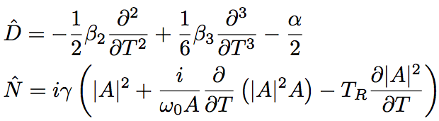 (Eq.2.5.28)(Eq.2.5.29)
in general case, the dispersion and the nonlinearity appears at the same timea along the fiber axial direction. In the split step Fourier method, assuming that the dispersion effect and the nonlinear optical effect appears separately when light travels for a short distance, h, in an optical fiber, an approximated solution is calculated. More concretely, the light propagation from z to z+h is considered as the following three steps. Fig.2.29 shows the schematic of three steps.
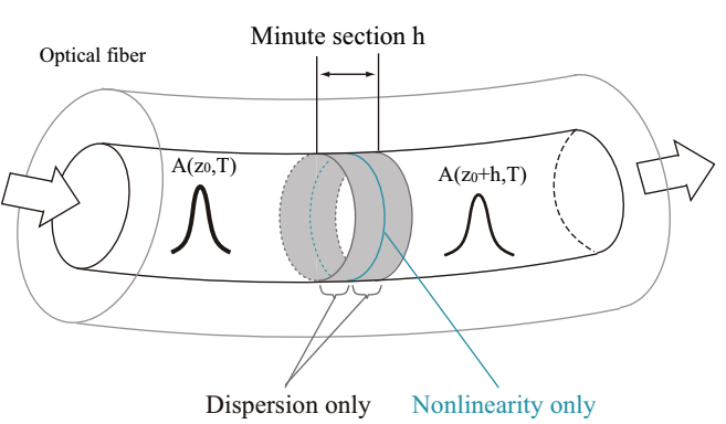
Fig.2.29 Split step Fourier method
① Assume that only the dispersion effect appears in the first region of the tiny interval, h, and consider the light propagattion for N^=0 in Eq.2.5.27. ② Assume that only the nonlinear optical effect apprears at the center of tiny interval and D^=0, and operate the nonlinear optical effect corresponding to the whole interval, h. ③ Consider that only the dispersion effect works at the remaining interval of h/2. These steps are expressed by the following equation.
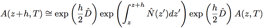 (Eq.2.5.30)
At first, assuming that a pulse propagates only by 2/h in the tiny interval at the begining, the exponential operator, exp(jD^/2), is operared in the Fourier space as shown below.
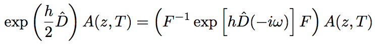 (Eq.2.5.31)
In Eq.2.5.31, F is an operator for Fourier transform, and D~(-iω) is an alternative of the differential operator shown in Eq.2.5.28 (∂/∂T is alternated by -iω). ω is a frequency in the Fourier space. Since ∂/∂T is just a figure in the Fourier space, Eq.2.5.31 can be directly calculated. By using an FFT algorithm, a numerical calculation of Eq.2.5.31 can be performed rapidly.
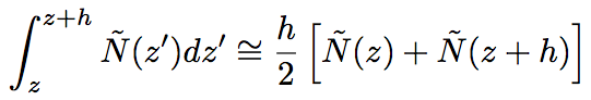
Second, the nonlinear optical effect corresponding to the whole interval is operated at the center of tiny space, h. As shown in Eq.2.5.30, the integral over the whole interval is operated. By utilizing a pedestal approximation, a precise approximation solution is obtained as shown below.
 (Eq.2.5.32)
However, since N~(z+h) is not obtained at the center, z+h/2, it is difficult to utilize Eq.2.5.32 without any modification. For the integral calculation, an iteration is used with setting a initial of N~(z+h) as N~(z). A(z+h,T) is derived from Eq.2.5.30, then a new value of N~(z+h) is calculated. Although the iteration calculation requires a long time, the calculation method based on this algorithm gives a result with a high accuracy. By using a larger interval step, h, the total calculation time becomes relatively shorten. In practice, twice iteration calculations are quite enough. Finally, assuming the propagation in the remaining h/2 region with considering only the dispersion, A(z+h,T) is derived.
In utilizing the split step Fourier method, we have to pay a lot of attentions to total time range, temporal resolution, propagating step range, and so on. Especially, the total time range has to be sufficently large with considering a time delay among each frequency component through the propagation. This is because a component reaching at the boundary of total time range is automatically input at the opposite side, resulting an instability of numerical calculation. We also have to be careful of the relationship between the total time range and the resolution of spectrum domain (Fourier space).
The temporal resolution has to be sufficiently better than a duration of propagating pulse. The optimal value of propagating step range depends on a complexity of issue. In case a large nonlinear optical effect is operated, a small propagating step range is required. Thus, by setting appropriate parameters, the split step Fourier method becomes the powerful analytical tool.
6. Polarization maintaining fiber
When light propagates in a birefringent material, the polarization of light is modified. The birefringence is a material property that a refractive index depends on the poratization of iight. In a single mode fiber (SMF), birefringence is randomly generated by strains in the fiber core and by some external stresses (environmental temperature change, mechanical vibration, etc…), although an SMF has a circular section and can transmit arbitrarily polarized light. When the SMF moves even slightly, the polarization in the SMF is changed by yielded birefringence. As a result, undesirable phenomena, such as the polarization mode dispersion (PMD) and an extraordinary connection with polarization-dependent device (ex. modulator), may occur with the SMF.
In order to avoid the polarization fluctuation, then to stabilize the polarization, a phase or polarization controller must be inserted and coiledefully aligned in the resonator. For the sake of polarization stability, the polarization maintaining fiber (PMF) was developed. If the polarization maintaining (PM) is not applied, the fiber laser is typically unstable against the environmental temperature change and mechanical vibration.
In this section, polarized light will be first explain, then PMF will be described.
6.1. Polarized light
Let us consider light at the orthogonal section against the propagating direction. If the electric and magnetic field is directed in one direction, the light is called as polarized light. Spontaneous light such as sunlight is not polarized light, while laser light is polarized light. The thought of polarized light is important for ideas of light propagation in an optical fiber. Fig.3.1 schematically shows polarized light (linearly polarized light composed of a couple of orthogonal rays).
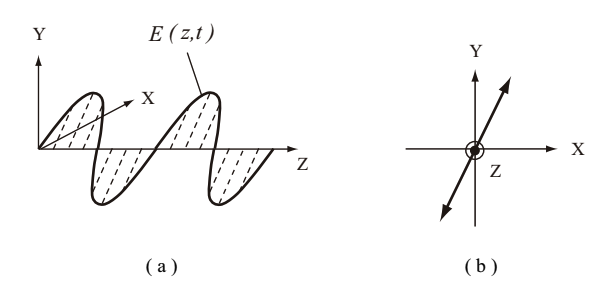
Fig.3.1 Linearly polarized light composed of a couple of orthogonal rays, Ex and Ey
Linearly polarized light in the (a) Y-Z plane and (b) Z direction
Even in an SMF, there exists not only a single mode, but a couple of linearly polarized orthogonal modes, LPxo1 and LPy01, can propagate. For the ideal SML with a perfectly circular core, the couple of modes are degenerated and their propagating constants are not identical in the case external force is not applied. However, for realistic SMF with imperfectly circular core, external heat, and mechanical stress, modal degeneracy is solved, and the polarization components are randomly mixed. Beacuse of this, the polarization is not maintained between at input and output edge. The linearly polarized light is changed to elliptically polarized light by a typical SMF due to the phase difference because the propagating constants are different.
Linearly polarized light
At first, let us consider the linearly polarized light. As the light wave propagates, it looks curving when seen at Y-Z plane. If the light wave is seen at X-Y plane, it looks fluctuating on the vertical line as shown in Fig.3.2. The polarization is decided by the vector direction and phase of electric field. Provided that the wave is projected to X- and Y-axis, the polarization is defined by the linear sum of X- and Y- axial components (Ex and Ey). In case these components propagates in one direction with the same phase, the light is linearly polarized light.
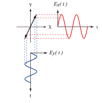
Fig.3.2 Schematic of linearly polarized light
Circularly polarized light & Ellptically polarized light
We have circularly polarized light and ellptically polarized light other than the linearly polarized light. Provided that the amplitude of Ex and Ey vector components are the same while the phases are different by 90 degree (that is, the amplitude is the maximum for one, while zero for the other), the light is circularly polarized light. When the amplitude and phase of Ex and Ey vector components are arbitrary, the light is elliptically polarized light. Fig.3.3 schematicaly represents the circulaly polarized and elliptically polarized light. The linearly polarized and circularly polarized light are special cases of the elliptically polarized light.
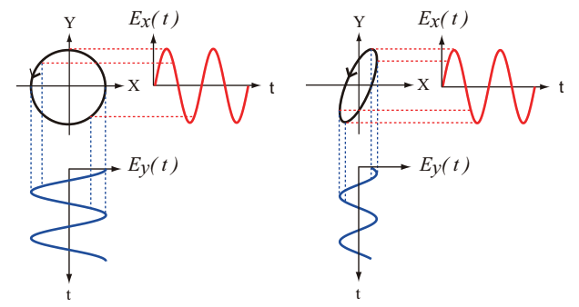
Fig.3.3 Schematic of circularly and elliptically polarized light
6.2. Property of PMF
An PMF is often called as a birefiringent fiber, and is purposely designed so that it is highly birefringent in order to suppress a random fluctuation of birefringence, which yields modulations of the light polarization. The birefringence is often induced by applying non-axisymmetric stress to the fiber core. This type of optical fiber is called as stress-inuced PMF. There are several types of stress-inuced PMF as shown in Fig.3.4; polarization-maintaining and absorption-reducing (PANDA) fiber, elliptical jacket fiber, and bow-tie fiber.
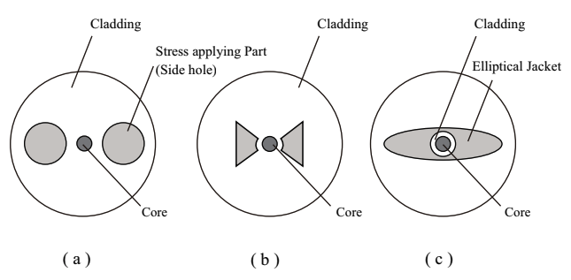
Fig.3.4 Section of kinds of PMF
(a) PANDA, (b) Bow-tie, (c) Elliptical Jacket
The stress-induced PMF has a nearly circular core, while a structured PMF has a non-axisymmetric core (elliptical core fiber). Various types of structured PMF have been suggested. The PANDA fiber, developed by the communication institute in Ibaraki, NTT, is currently mainstream since it is superior in the polarization crosstalk property, and is relatively a low-loss fiber. The characteristic of PMF, especially of PANDA fiber, will be described in the following items.
6.2.1. Fast axis and slow axis
Because an PMF is highly birefringent, the group velocity of light is different in a couple of orthogonal axes. For a small modal index, the group velocity of light propagating in the mode direction is large The mode direction is called as fast axis. An axial direction which has a large modal index is called as slow axis. Fig.3.5 shows a section and a distribution of refractive index of PANDA fiber.
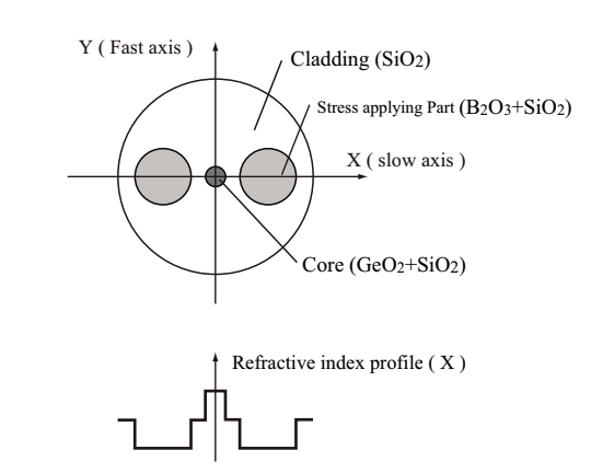
Fig.3.5 Fast and slow axis of PANDA fiber
In a PANDA fiber, a tensile stress is applied in the X direction, while a compressive stress is applied in the Y direction. As a result, a photo-elastic effect induces birefringence. Therefore, a difference in refractive indices effectively working on the polarization (effective modal index) bewteen X and Y direction (nx, ny) is yielded. This makes a diffrence in the propagating constants between X polarizaion (slow axis) mode and Y polarization (fast axis) mode, Bx and By, then a coupling between a couple of polarization modes becomes difficult. The amount of modal birefringence, B value, is defined by the following equation.
The wavenumber is k0=2π/λ
6.2.2. Polarization cross talk
Provided that linearly polarized light is input in the polarization mode of either fast or slow axis, polarization crosstalk is represented by quenching ratio of orthogonal polarization modes at output edge; one is the polarized mode in the input direction, and the other is the leakig polarized mode in the orthogonal direction, as given by the following equation,
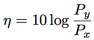 (Eq.3.1.2)
where Px, and Py is the power of light in X, and Y direction, respectively. The larger the birefringence is, the smaler the polarization crosstalk is, and the better the polarization maintaining property is. As light propagates in the fiber, the optical coupling occurs between polarization modes. Therefore, the polarization crosstalk is a function of the fiber length (in theory, linear function). The unit is “dB/100.” The standard requirement is -25 dB/100m or lower.
The polarization crosstalk of PANDA fiber is little temperature-dependent in the range of -40 ~+80 degree. Additionally, the polaization crosstalk of PANDA fiber is not degraded by torsion and bending, which may be applied in typical uses.
6.2.3. Beat length
When the polarization direction of incident light corresponds to either of the fast or slow axis, the polarization direction of propagating light in the fiber does not change. However, the polarization direction of incident light is tilted against both the fast and slow axis, the polarization changes continuously since the light power is periodically exchanged between X and Y polarized modes of PMF. The phase difference between the propagating X and Y polarized light can be 2π at some distance. The distance (for the polarization to return to the original) is called as beat length, Lb, or coupling length.
Fig.3.6 schematically shows the series of polarization change in PANDA fiber when a linearly polarized light is incident along the direction tilted from X (or Y) polarized light by 45 degree.
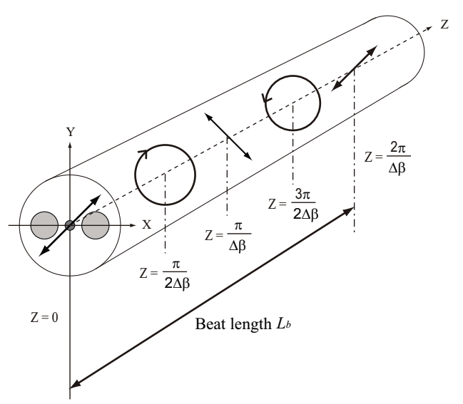
Fig.3.6 The series of polarization change in PANDA fiber when a linearly polarized light is incident along the direction tilted from Fast axis by 45 degree.
The beat length represents the amount of birefringence. The relationship between beat length, Lb, and birefringence, B, is expressed as follows.
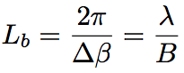 (Eq. 3.1.3)
6.2.4. Cut-off wavelength & mode field diameter
Since PANDA fiber is a type of SMF, cut-off wavelength and mode field diameter (MFD) are the important properties as well as propagation loss.
Since the distributions of refractive index for X and Y polarized light in the PANDA fiber are different each other, there are a coupld of cut-off wavelengths. For the X polarized light, the equivalent refractive index is higher and the cut-off wavelength is longer. In a typical PANDA fiber, the cut-off wavelength for the X polarized fiber is indicated so as to use either of cut-off wavelengths.
MFD is slightly different between the X and Y polarized light.
6.2.5. Bending loss
When an PMF is bent, the Y polarized light is more likely to be degraded, since the equivalent refractive index is smaller, compared with the X polarized light.
6.2.6. Fusion splice
For fusion splice of PMF, in addition to aligning as well as for a non-PM fiber, angle tuning by rotating fiber is necessary for aligning polarization axis. Since the fusion loss depends on MFD and the core eccentricity beween fibers, the fusion loss for PANDA fiber can be as small as a non-PM fiber. However, the polarization crosstalk increases when the angle bewteen polarization axes is mismatched. Recently, since a fiber fusion splicer for PMF is commercially available by using an appropriate splicer, a good fusion splicing without an increment of polarization crosstalk is possible.
6.2.7. Rare earth doped PMF fiber
Rare-earth-doped single mode PMF and ytterbium-doped double clad PMF are employed in a fiber laser oscillator and fiber laser amplifier.
7. Double clad fiber
For fiber laser which is used before 1980s, a pump laser is directly irradiated to the fiber core for pumping (fiber laser with direct cre-pumping). Although the damage threshold of silica glass, the main component used in optical fiber, is as high as ~2GW/cm^2 @CW, high power pumping of SMF by the direct core-pumping was difficult in terms of both the technique and material (especially when spatial-output LD is used), since the core diameter is very small. In the case of using multi-mode fiber (MMF), the direct core-pumping distorts the beam quality, and is not usable for the processing, which requries high power and a good beam quality.
In 1988, a method for realizing high power fiber laser with a good beam quality was suggested. The fiber laser was double clad fiber (DCF) laser. DCF laser became common so fast. Nowadays, DCF is a mainstream method for pumping high power fiber laser. DCF can be adapted for large mode area fiber described in the following section.
7.1. Core-pumping and clad-pumping: comparison
The direct core-pumping of Yb-doped SMF, and clad-pumping of Yb-doped DCF are shown in Fig.3.7(a), and (b), respectively.
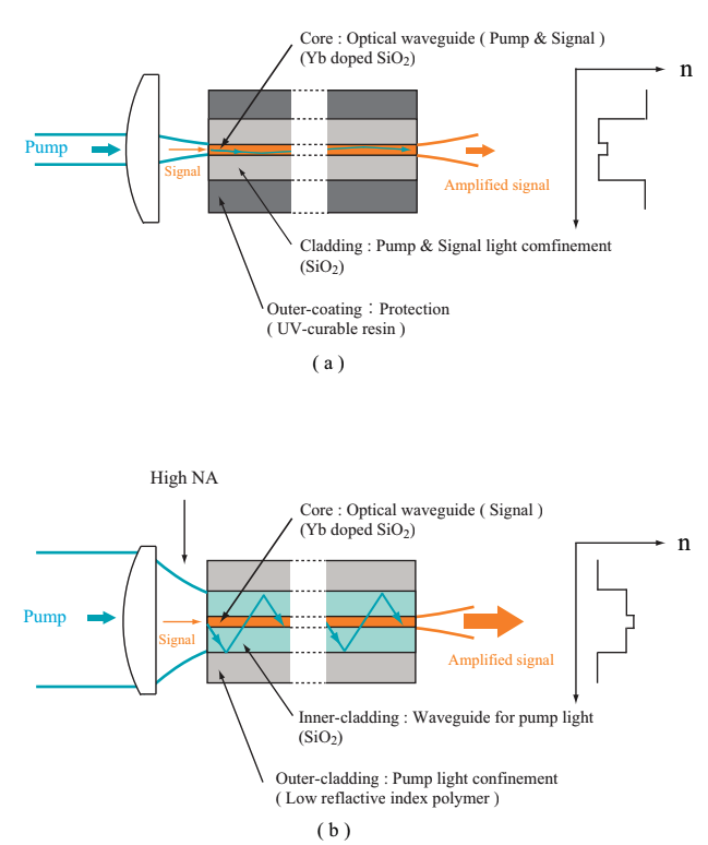
Fig.3.7 (a) Core-pumping with Yb-doped SMF and (b) clad-pumping with Yb-doped DCF
FIg.3.7(a) represents that pumping light propagates through and directly pumps the core. Fig.3.7(b) shows that pumping light propagates through the inner clad and pumps the core. The used optical fiber is DCF. DCF has a couple of clad layers.
The inner clad is often called as the first clad, while the outer clad is often called as te second clad.
The inner clad is composed of silica glass. The inner clad plays a role of clad, which confines the signal light propagating through the core, and also plays a role of multimode waveguide (multimode core) of the pumping light. Since the inner clad has a high NA (~0.46) and large cross-section (several hundreds µm in diameter), the power density of pumping light propagating in the inner clad is low. Therefore, the clad-pumping is effectively performed by multimode LD of which output power is high but beam quality is low. The outer clad is made of low-refracting polymer (resin material) and functions as a clad against the pumping light. SInce NA of the inner clad is better to be larger, DCF is designed to have a large difference in the refractive index between the inner and outer clad.
In the case that rare earth ion, such as Yb3+, is doped in the DCF core, the doped ion in the core is excited by the pumping light crossing over the core, and the signal light is amplified (energy conversion from the pumping light to the amplified signal). The amplified signal is confined in the inner clad, and propagates throught the core with a low NA and small cross-section. Since the NA of core is small, higher-order modes in the amplified signal is suppressed. The amplified light emitting from the core with a small NA and cross-section has a good beam quality and focusing property.
DCF plays a role of brightness converter, which efficiently converts the pumping light of LD with a low brightness to laser light with a high brightness. This is the essence of high power fiber laser, and is the essential difference from other solid-state lasers.
In uses of DCF, the clad-pumping with low coupling loss is possible when it is coupled with MMF pigtail LD having the equivalent core diameter to the inner clad diameter, or the pump combiner assembling the output of several LDs with the same fiber property (fusion splicing).
7.1.1. Brightness
The brightness of laser is defined by the following equation,
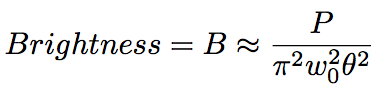 (Eq.3.2.1)
where P is the light power, w0 is the radius of beam waist, and θ is a half angle of far-field beam divergence. Provided the brightness of pumping light, BPump, and the brightness of laser light, BLaser, the ratio of BLaser to BPump is smaller than 1 for the direct core-pumping fiber laser, while it is given by the following equatio for the clad-pumping fiber laser,
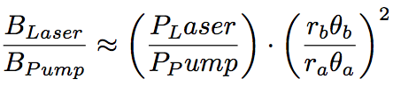 (Eq.3.2.2)
where ra, rb is core radius, inner clad radius, respectivel, and we have θa = arcsinNAcore, and θb = arcsinNAinner-clad (NAcore is NA of core, and NAinner-clad is NA of inner clad). For a typical clad-pumping Yb fiber fiber laser, BLaser/BPump can be larger than 5000.
7.2. Efficient pumping
Absorption efficiency of pumping light largely affects the total efficiency of oscillation in a fiber laser with quantum yield close to 1. Therefore, structure of DCF must be appropriate for the efficient pumping with high power pumping light.
For the round-shape-section coaxial clad, which is typically used and is easy to manufacture, in case the pumping light does not input at the core edge, it propagates with helically circlinginside the inner clad (skew) without crossing the core, as shown in Fig.3.8(a). As a result, the pumping light can not contribute to the pumping. As the core cross-section to the inner clad cross-section ratio decreases, the skewing component increases, resulting in lowering of the pumping efficiency.
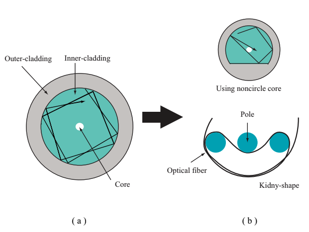
Fig.3.8 The efficient pumping with DCF
(a) Skew in round inner clad and (b) highly efficient pumping method
In order to scatter the skewing component, the sectional shape of inner clad is specialized as shown in Fig.3.9. As represented in Fig.3.8(b), when DCF is bent toward kidney-shape, spatial mode mixing occurs, then the more efficient pumping becomes possible. Since the kidney-shape DCF gives a large bending loss to the higher-order modes of laser traveling in the low NA core, it is employed for collecting the energy from MMF to the output of fundmental mode.
In a non-circular inner clad, mode is continuously converted during the propagation. The incident pumping light is efficiently absorbed by the core in case the fiber length is long. Fig.3.10 represents the relationship between a sectional shape and absorption characteristics of inner clad of DCF. Except for the case of circular section, the absorptivities are all similar each other for sufficiently long fiber. An regularly octagonal or D-letter-shape inner clad is typically utilized because they has the large pumping efficiency. Since the regularly octagonal inner clad is symmetric, the fucion of optical fiber is easy, while manufacturing is difficult. The D-letter-shape inner clad is easy to manufacture, but has a difficulty in the fiber fusion due to the ansymmetry.
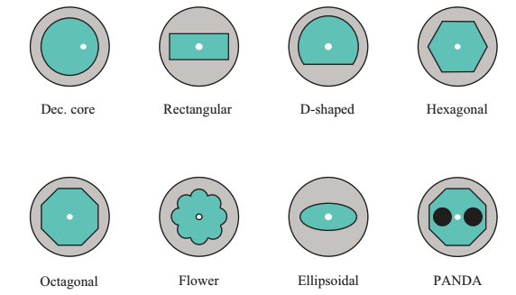
Fig.3.9 The sectional shape of inner clad of DCF
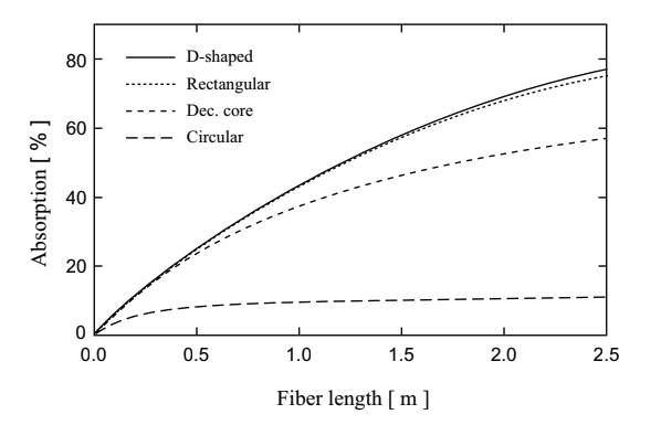
Fig.3.10 The relationship between a sectional shape and absorption characteristics of inner clad of DCF
8. Large Mode Area Fiber
When high power laser prppagates in optical fiber, the nonlinear optical effect, such as stimulated Raman scattering (SRS) and stimulated Brillouin scattering (SBS), may occur. The nonlinear opitcal effects limit the property of high power fiber laser. To avoid the nonlinear optical effect, either of an optical fiber with the large core diameter and a short-length optical fiber is necessary. In a short-length optical fiber, since the interaction length is short, the efficiency of fiber laser is low. To suppress the nonlinear optical effect with keeping the high efficiency, an optical fiber with a large mode area (mode field) is required. Large mode area (LMA) fiber that is designed to have a low NA and large diameter was developed under this rquirement. LMA fiber is typically a DCF as is understood by the reason for its development. The difference between a typical DCF and an LMA DCF can be seen in Fig.3.11.
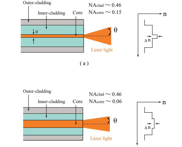
Fig.3.11 (a) a typical DCF and (b) an LMA DCF
In a typical SM fiber for fiber laser at 1064 nm, the MFD is ca. 6 µm, and the mode area is ca. 30 µm^2. On the other hand, in the LMA fiber for high power fiber laser with 30 µm core diameter, MFD is ca. 2 µm, and the mode area is ca. 450 µm^2. Because of the larger mode area, in a CW fiber laser, the threshold of SRS for the LMA reaches up to kW range, while one for the SMF is ca. 100W. In a pulsed fiber laser, the SRS threshold for the LMA is ca. 300kW (peak power), while one for a typical SMF is ca. 20kW.
At an SM propagation in SI-type fiber, the relationship between the core diameter, d, and the core NA is represented as follows.
 (Eq.3.3.1)
According to this equation, the NA must be small when the diameter is large. For example, a perfect SM is obtained at NA = 0.038 or lower for 20 µm core diameter, or at NA = 0.025 or lower for 30 µm core diameter. The lower the NA is, the larger the bending loss of fundamental mode becomes, consequently, a long-period stability and reproducebility is reduced. A typical LMA fiber is an MMF, but not an SMF. The core diameter is in the range of 10~40 µm, and the NA is ca. 0.06. For instance, the following configurations are employed.
….
In Fig.3.12, an optical amplifier composed of Yb-doped LMA DCF (the second configuration) is represented.
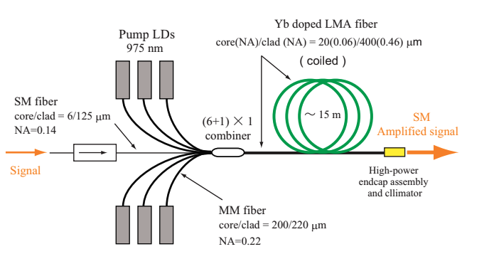
Fig.3.12 An optical amplifier composed of Yb-doped LMA DCF
Rare-earth-doped optical fiber is called as active fiber, while non-doped fiber is called as passive fiber. Passive LMA fiber enables low-loss transmission of high energy light, therefore, is applicable to high power laser transmission, pump combiners, and sensor probes. The passive LMA fiber having the same core diameter and NA with an active LMA fiber is often used for fiber laser and optical fiber amplification. LMA fiber is not always SI-type, but some are photonics crystal fiber type.
8.1. Linear polarization mode control
In a typical SI-type optical fiber, the spatial mode number, N, is expressed as N~V^2/4, provided that the degree of freedom of polarization is excluded. For NA = 0.06, and the wavelength of 1064nm, N is obtained as N=3,7,78, and >300, at the core diameter of d=20,30,100, and 200µm, respectively.
In the electric field distribution of light with multimode propagation, the higher-order mode leaks from the core to the clad (see Fig.2.5). By bending the optical fiber, the bending loss of higher-order mode is enlarged without increasing the bending loss of fundamental mode. Since NF is as small as 0.06 for an LMA fiber, giving a large curvature can control linear polarization (LP) mode. As a result, a good beam quality (nearly single mode: M^2~1) is realized (mode filtering effect).
Coiling an LMA fiber is well-known method for suppressing higher-order modes. Fig.3.13 shows the relationship between the curvature radius and bending loss in the initial four transverse modes for the coiled LMA fiber with core diameter of 30µm and NA=0.06. For the fiber curvature radius of 5 cm, the bending loss of LP01 mode is ~0.01 dB/m, while the bending loss of LP11 mode is ~50dB/m. This LMA fiber enables the SM propagation of laser light when it is bend with the curvature radius of 5 cm.
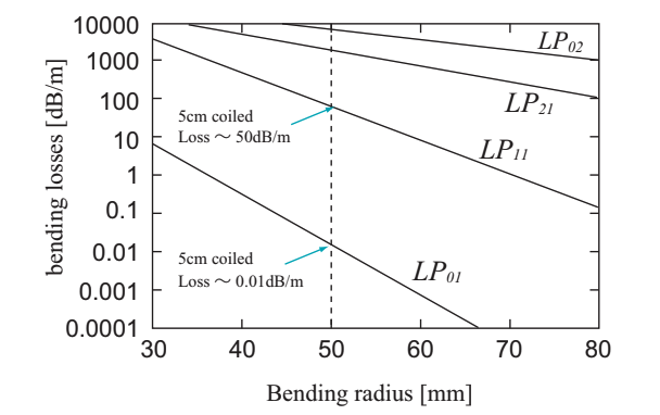
Fig.3.13 The relationship between the curvature radius and bending loss
The singlemode output power exceeded 1kW in 2004 (the previous maximal power was 100W). This achievement attributes to the development of LMA fiber and high power semiconducting laser. Nowadays, 10 kW output is possible by using the setup shown in Fig.3.14. 15~20kW is expected in the future perspective. By using the LMA Yb DCF amplification with the core diameter of 80 µm and NA=0.06 and suppressing the nonlinear optical effects, SM output with peak power of 1.6MW, pulse duration of 700ps, pulse energy of 1mJ, and repetition rate of 50Hz was realized.
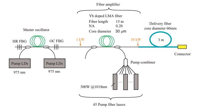
Fig.3.14 Configuration of 10kW singlemode fiber laser system
8.2. New types of LMA fibers
In LMA fiber, the mode area is controlled by the difference in refractive indices between the core and clad, Δn. In a typical SI-type LMA fiber, however, because of the limitations of modified chemical vapor deposition (MVCD) and direct nanoparticle deposition (DND) techniques, it is difficult to control the core-clad difference in refractive indices far below 10^-3, therefore is difficult to manufacture low NA (<0.06) optical fiber.
To overcome the difficulties, a perfect SM LMA fiber (mode cross-section~2000µm^2) was developed by controlling the interval of periodic holes and diameter in photonic crystal fiber (PCF), which perfectly controls low NA value, as a new-type technique. However, if the NA is too low, the propagation property is sensitive not only to macroscopic bending, but also to mciroscopic bending loss. Therefore, the length of LMA is limited.
Rod-type PCF Rod-type PCF is developed to avoid increases in the bending loss accompanied with low NA, which is realized in PCF. The rod-type PCF can not be bent. The core diameter of PCF is 60~100µm. In order to keep the fiber being straight, the rod-type PCF is supported by the quartz tube (outer clad) with a diamter of ca. 2mm. By september 2010, the rod-type PCF with mode area of 4500µm^2 (Yb-doped, polarization maintaining, core diameter of 100µm, pump-clad of 285µm, outer-clad of 1.7mm) is commercially available as a rod-type PCF with the maximal mode area. This rod-type PCF has a nearly 100 times larger mode area than a typical SMF.
So far, a rod-type Yb-doped LMAPCF achieved a femtosecond chirped pulse amplification (CPA) with an average power of 131W, pulse duration of 220fs, and peak power of 8.2MW(@73MHz).
CCC fiber Chirally-coupled core (CCC) fiber has a coiling structure of passive site core around the rare-earth-doped centering core (core diameter of 35µm, NA=0.07) as shown in Fig.3.15. In a CCC fiber, higher-order modes are strongly coupled with the side core, while the most of fundamental mode travels in the core center. The higher-order modes are largely affected by the bending loss (the loss is 90~130dB/m) in the side core, and finally LP01 mode remains in the core center (the loss is 0.2~0.3dB/m). Master oscillator power amplifier (MOPA) system using Yb-doped CCC fiber with the core diameter of 35µm realizes 100kW peak power at 100kHz repetition rate with 100W average power and 10ns pulse duration. With using CCC fiber, a fiber laser with pulse energy of 1.0mJ at 10~100kHz, pulse duration of 10ns, average power of 100W, and beam quality of M^2<1.1, and SM propagation in the core diameter of 50~100µm are expected.
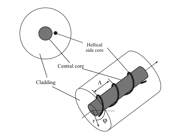
Fig.3.15 Configuration of CCC fiber
9. Photonic crystal fiber
Photonic crystal fiber (PCF) is a type of optical fiber, and has periodic structure of holes in quartz. The first attempt of aligning holes in optical fiber is in 1973. The purpose of hole alignment in optical fiber was to minimize the transmission loss at that time, but the transmission loss of silica glass fiber was dramatically suppressed by another method. The structure of currently used PCF is based on the suggestion in 1996.
3.4.1 Sorts
PCF is categorized into two types by waveguiding principles. One is a photonic band gap fiber (PBF), a photonic band-gap PCF. PBF has two-dimensional Bragg reflection structure, and allows light to propagate in the air core. Light with a specific wavelength can not penetrate in the medium, in which air holes are aligned with a period close to light wavelength, with large change in the refaction index, while light with different wavelength can penetrate the medium. The restrict structural periodicity and hole size homogenuity are required for manufacturing PBF. The other type of PCF is index guiding PCF, and is also called as micro-structured fiber. The both types control brand-new propagation properties by forming periodic microstructure in a wavelength order in the optical fiber.
Fig.3.16 schmatically rpresents the section of various types of PCF. FIg.3.16(a-c) shows the index guiding PCFs; (a) is a typical one, (b) simplifies (a) and is used in the case that some limited properties are required, and (c) dopes impurity such as Ge as well as a normal fiber and is used especially for suppressing the bending loss. Fig.3.16(d) is PBF and is used for the communication with short wavelength, UV range, which does not propagate in the previously used quartz fiber, or high power transmission, since the core, the part that light propagates in, is the air.
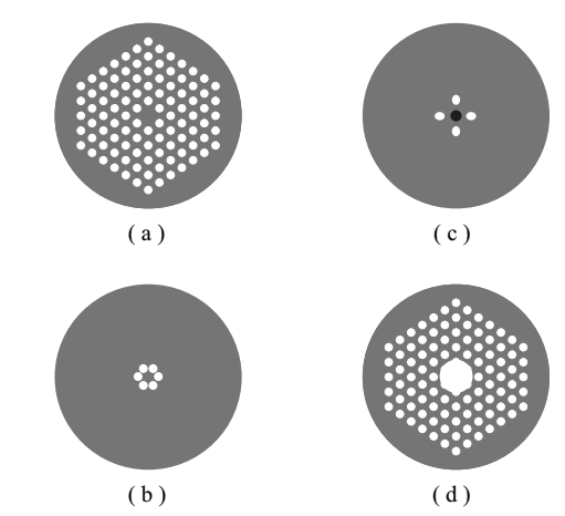
Fig.3.16 The section of various types of PCF
The commercially available PCFs are briefly described below.
(1) Hollow core PCF, PBF In a general optical fiber, the core part where light propagates is composed of quartz glass. In the hollow core (HC) PCF, since the core is filled with air, the fiber is hardly damaged, and nonlinear properties are avoided. HC-PCF will be applicable to long-distance transmission since it has little nonlinearity.
(2) LMA PCF In a general fiber, light exhibits multimode propagation when MFD is large. On the other hand, an LMA fiber allows singlemode propagation in spite of the large MDF. Since the MFD is large, LMA PCF is not affected by the nonlinear property and the material damage. Therefore, the high-power light transmission is possible with LMA PCF.
(3) Highly nonlinear PCF In a general optical fiber, the nolinear coefficient is small, and the wideband light is not generated. In a highly non-linear (HNL) PCF, since the nolinear coefficient is large, supercontinuum (SC) light extending in the visible and near-infrared range is generated.
(4) Endless single mode PCF In a general SMF, light with shorter wavelength than the cut-off wavelength exhibits multimode propagation. On the other hand, in the endless single mode (ESM) PCF, light can exhibit singlemode propagation regardless of the wavelength and the core diameter.
(5) PM PCF In a general PM fiber, the stress yields birefringence, and the birefringence maintains the polarization. In a PM PCF, a large difference in refractive indices between air and glass, and the elliptical shape yields a large birefringence. Compared with a general PM fiber, since the beat lengh is shorter, the polarization is less disturbed by the bending and the temperature change.
9.1. Analysis & manufacturing
PCF can be analyzed by effective-refractive-index method, multipole method, local mode expansion method, finite element method (FEM), finite difference time domain (FDTD) method, and so on.
Let us consider the fundamental configuratoin of single defect core/triangular lattice clad shown in Fig.3.16(a). Based on the core-clad system, typical structural parameters of PCF are explained below. Provided the air hole pitch, Λ, the air hole diameter, d, as shown in FIg.3.17, the core diameter, D, and the porosity, F, are expressed by the following equations.
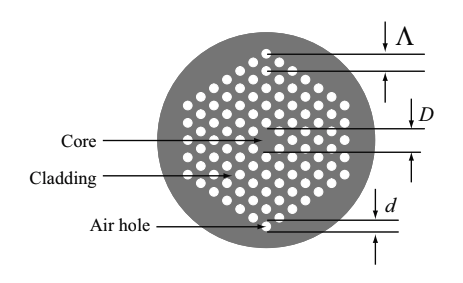
Fig.3.17 The section structure of PCF
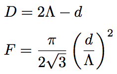 (Eq.3.4.1)(Eq.3.4.2)
The porosity, F , is the rate of air to highly-refractive medium. The ratio of air hole diameter to to the pitch, d/Λ, is often used as a standardization parameter of structure, since d/Λ is relevant to effective refractive index of the clad.The ratio of pitch to the wavelength, Λ/λ, represents the standardization frequency. By appropriately tuning these parameters, we design various types of optical fibers, featured by wideband SM operation, high nonlinearlity, polarization maintaining, or low bending loss, superior to a typical one. In PCF, the refractive index difference between core and clad, the effective refractive index, can be tuned relatively freely and largely compared with a typical optical fiber.
In manufacturing PCF, general methods such as modified chemical vapor deposition (MCVD) method and vapor-pjase axial deposition (VAD) method are not available, since PCF has air holes. Stack-and-Draw (capillary) technique and drilling technique are often used. Refer to the citation fot more details.
9.2. Treatment
This section describes cautions in uses of PCF. Whe the edge face of PCF is open, air with high moisture enters the air holes, which may yield increases in the transmission loss, enhancements of temperature dependency of the transmission loss, and contamination at the edge face. In addition to these problems, the edge face becomes easy to be damaged. In case the femtosecond pulsed laser is used, the edge face of core with a small diameter is easily damaged, since the laser peak intensity is high.
To avoid this kind of damage on the edge face, edge face sealing is used for PCF. By closing the air holes with heat treatment of the fiber edge face, air with high moisture can not get into the air holes. Additionally, by incresing the spot size at the edge face (MFD) and NA, the damage threshold for the edge face is increased. As results, connector splicing, polishing, and coating become possible.
(1) Fusion splice of PCF Low-loss fusion splice of PCF with a normal optical fiber is necessary in some cases; light emitting from PCF is detected or measured; PCF is connected with another light source; all-fiber-type light source is constructed. However, the low-loss fusion splice is difficult because PCF has a lot of air holes. When the PCF fusion splice is performed, the air holes are destroyed owing to the arc discharge by the fusion splicer. Therefore, the light is not confined in the core, then light propagating in PCF leaks at the splicing site, resulting in the large loss. Additionally, Fresnel reflection remarkably occurs due to the difference in refractive indices of the clad sites.
To avoid the fusion splicing loss, an optical fiber with the same MFD as PCF is connected. When an SMF with 6µm MFD is connected with PCF having 20µm MFD, the light leaks out of the fiber, resulting in the large loss. Pigtail fibers and bridge fibers are utilized for mode-matching.
10. Pumping light source – Laser diode (LD)
Semiconducting laser (LD) is the most important component in the system of high-power fiber laser. Oscillation wavelength of LD depends on a type of atom composing the semiconductor. Table 4.1. shows the atoms of semiconductor, corresponding ranges of oscillation wavelength, and types of rare earth doped fiber which can be excited at each wavelength range. As is indicated by the table, LD is applicable to wide frequency range.
Table 4.1: Atoms of semiconductor, corresponding ranges of oscillation wavelength, and types of rare earth doped fiber which can be excited at each wavelength range
| Constituent element | Wavelength range [μm] | Rare earth |
| InGaN / GaN | 0.38-0.48 | Pr |
| GaAs / AlGaAs | 0.78-0.86 | Nd, Tm |
| InGaAs / GaInAsP / GaInP | 0.9-0.98 | Yb, Er |
| GaInAsP / InP, AlGaInAs / InP | 1.47-1.6 | Er |
| InGaAsP | 1.8-1.96 | Ho |
10.1. Fiber-coupled LD configuration
LD is employed as a pumping light source for the typical fiber lasers. LD is typically treated as a module intergrating optical fiber. For the purpose of pumping of fiber laser and optical amplifier, a 14-pin butterfly package is often used.
A typical 14-pin butterfly package is a single-emitter-type, and is composed of an LD chip, a beam isolater, a thermoelectric cooler (TEC), and a photodiode (PD) for monitoring the laser power or wavelength. Laser output is generated from the optical fiber equipped with ferrule.
An LD chip emitting light is attached via a sub-mount to a Peltier device (TEC) which is for temperature control. Laser light emitted from the LD chip is focused into optical fiber (single-mode, multi-mode, polarized-wave maintaing, large diameter, etc ) by a micro-lens. A monitoring PD (such as a p-intrinsic-n photo diode) can check the laser output power. These devices are fixed by YAG laser welding after a precise position adjustment.
For the pumping of fiber laser, a fiber pigtail LD is employed. Table 4.2 summarizes different types of the fiber pigtail LD. Single-mode fiber (SMF) pigtail LD can be used for fiber fusion with SMF, and is mainly used for the pumping of rare earth doped SMF. Multi-mode fiber (MMF) pigtail LD can be fused with a pumping port of pumping combiner, and is mainly used for the pumping of rare earth doped double-clad fiber (DCF).
Table 4.2: Different types of the fiber pigtail LD and maximum power at CW
| Types of LD | Types of fiber | Core diameter | Maximum power @CW | Reference |
| Single-emitter-type | SMF MMF |
~10μm ~100μm |
0.8W ~25W |
6) 7) |
| Bar-type | MMF | ~100μm | ~30W | 8) |
| Stack-type | MMF | ~600μm | ~400W | 9) |
10.1.1. Cautions for uses of LD
In preparing an LD for constructing a fiber laser, a connection drawing must be checked, and a mount and TEC controller for a package is necessary to be appropriately selected. Discharge of static electricity needs to be avoided, for example, by equipping an electro-static discharge (ESD) wrist strap, because LDs are easily broken by the static electricity.
10.2. Spectral stabilization
In a Peltier device, a pair of n-type and p-type semiconductors are sandwitched by two types of metal. The Peltier effect transfers heat and cools down an object. The Peltier device is effective for thermal control with high accuracy and local cooling. The Peltier device is employed to control the temperature of LD with an accuracy of 0.01 degree or more with detecting temperature around the LD by thermistor. In LD, the oscillation wavelength depends on the temperature (~0.1nm/degree).
In LD module for pumping in optical amplifiers, such as Er-doped fiber amplifier (EDFA) and Raman amplifier, fiber Bragg grating (FBG) is attached to pigtail fiber. The oscillation wavelength is fixed into the blaze wavelength of FBG, even when driving current and environmental temperature of LD change. Consequently, the oscillation spectrum is sharpen (0.1~several nanometers at 95% output power) and stabilized (~0.01nm/degree at FBG temperature).
(1) Reguirements for the pupmping light source Low electricity consumption (= high efficiency) and high output power (400 mW or higher) are required for the specification of pumping light source for fiber laser. For polarization maintained (PM) laser, then, PM fiber (PANDA) is necessary.
The requirement depends on the application. For instance, the Raman amplifier requires, in particular, wavelength stability (fluctuation of the osciilation wavelength causes fluctuation of gain wavelength range), spectral sharpness of oscillation line (broad oscillation line yields a large wave mixing loss in the wavelength-mixing coupler, and increases the number of longitudinal mode in the oscillation line, resulting in a noise and gain fluctuation caused by the oscillation of a number of longitudinal modes), low relative intensity noise (RIN, intensity fluctuation of the excitaiton light results in fluctuation of the Raman gain because an amplification process in the Raman amplifier is fast), and longitudinally multi-modes (when high power light is focused in the narrow wavelength range, the pumping efficiency decreases due to stimulated Brillouin scattering), of the pumping light source.
11. Gain medium – rare earth doped fiber
A rare earth doped fiber, in which trivalent ion of rare earth (RE) is doped into the core as an active material, has transition lines in the wavelength range below 3µm as shown in FIg. 4.3. A doped amount of typical RE ion, Er3+, Nd 3+, and Yb3+, is 100 ppm (part per million) or more (10,000 ppm (1%) or more). RE ion is incorporated into RE2O3 in the silica glass. For the high doping concentration, an RE distribution can be clustered (clustering). The clustering can be avoided to some extent by doping Al2O3, P2O5, or so on together, which makes RE ion easily melt. Doping of Al2O23 also smooths and expands the fluorescence spectrum. In order to increase the refractive index, GeO2 is added into the core.
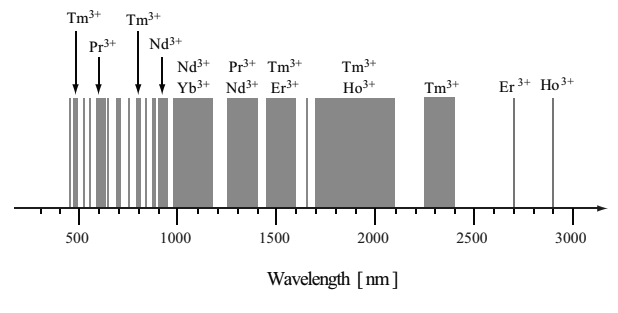
Fig.4.3 Luminescence wavelength range of rare earth doped fibers
In this section, we describe the characteristics of rare earth doped fiber. Rare earth doped fiber is employed for Yb fiber laser and Er fiber laser, which is used in general. In particular, Yb doped fiber is explained in detail. Fig. 4.4 shows Yb3+, Er3+. and Tm3+ energy structures, which principally contribute to the laser oscillation.
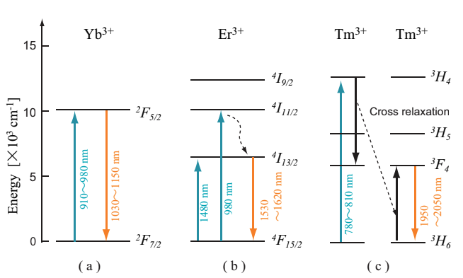
Fig.4.4 Energy level diagrams of rare earth ions
(a) Yb3+, (b) Er3+ and (c) Tm3+
(1) Ionic interaction When an optical fiber contains of a different or the same kinds of rare earth ions with high concentration, energy transfer with or without luminescence can occur among rare earth ions. In the energy transfer process, an ion, which emits the energy, is called a donor, while an ion, which receive the energy, is called an acceptor. The energy transfer can yield concentration quenching and intensified sensitivity.
(2) Tm doped fiber By exciting Tm doped fiber with ca. 793 nm light, Tm fiber laser oscillating at 2 µm range is obtained. Tm fiber laser is known as an eye-safe laser, because light in 1.4 ~ 2.6 µm range is hard to reach at the retina. In the 2 µm range, a biological cell or tissue has a local maximum of absorption by water, while there is an atomospheric window, in which the transmission property for the air is good). Therefore, Tm fiber laser is employed for medical laser mes, laser-based distance measurement system, light detection and ranging (LIDAR, lader system using light instead of radio wave), and range finder. In a recent Tm fiber laser, 53 % slope efficiency and 1kW or higher average power at 2045 nm is realized .
11.1. Yb-doped fiber
11.1.1. Spectroscopic property
The atomic number of ytterubium (Yb) is 70. Because the electronic arrangement of Yb3+ takes [Xe]4f13 structure, Yb3+ can only have a ground state 2F7/2 and an excited state 2F5/2. The energy structure of Yb silica glass is showin in Fig. 4.5 in detail. The ground state, 2F7/2, is composed of four of stark levels, while the excited state, 2F5/2, is composed of three of stark levels.
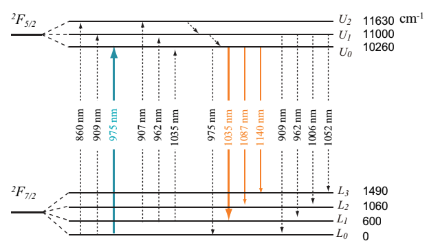
Fig.4.5 Energy level diagram of Yb silica glass
Absorption cross-section and stimulated emission cross-section
Absorption and stimulated emission cross-sections of Yb doped silica glass optical fiber (Yb fiber) are shown in Fig. 4.6(a). The absorption or fluorescence peak at ca. 975 nm (A) represents the zero-line transition between the lowest energy levels of the exicted state, 2F5/2, and ground state, 2F7/2, in manifold. The laser operation at the wavelength of ca. 975 nm is three-level because the emission is due to a transition to the lowest stark level. The absorption peak at shorter wavelengh (B) corresponds to a transition from the ground level L0 to either of the excited level, U1 and U2. The absorption peak at longer wavelengh (C) corresponds to a transition from the level L1 to the level U0.
Fig. 4.6(b) shows the aborption cross-section of Yb fiber at around 1000 nm in detail. The absorption of Yb fiber at (C) is relatively small, but it is an origin of gain loss by reabsorption of laser light and is important. The fluorescence having a peak approximately at 1030 nm (D) has a lower slope up to 1200 nm. The fluorescence corresponds to transitions from the laser upper state, U0, to the laser lower states, L1, L2, and L3. These transitions are seen as a four-states system. The fluorescence at (E) represents transitions from the level, U1, to the level, L0 or L1.
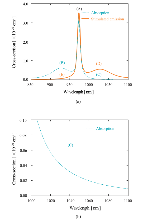
Fig.4.6 Absorption and stimulated emission cross-sections of Yb doped silica glass optical fiber
(a) Absorption and stimulated emission cross-sections of Yb doped silica glass optical fiber, (b) absorption cross-sections in the wavelength from 1000 nm to 1100 nm
(1) Comparison between 915 nm and 975 nm pumping The local maximums of absorption spectrum of Yb fiber are, as was shown in FIg. 4.6(a), approximately at 975 and 915 nm. Therefore, wavelength effective for the Yb fiber pumping can be either 975 or 915 nm. The comparison of property between 915 and 975 nm pumping is showns table 4.3. The pumping efficiency is lower for 915 mn pumping compared with 975 nm pumping, because the absorption is approximately three times smaller at 915 nm than 975 nm. Therefore, at 915 nm pumping, the gain fiber needs to be longer to obtain the same output power with the same pumping power as the case of 975 nm pumping. This means, at 915 nm pumping, nonlinear optical effects can be remarkable, while the cooling ability can be high due to the large fiber aspect ratio. For 975 nm exictation, a stability of the osciilation wavelength is important because the absorption band is narrow , while the wavelength stability is not essential for 915 nm pumping because the absorption band is wide. Even by taking account this issue, 975 nm pumping laser is superior because of the high efficiency and low running cost.
Table 4.3: comparison of property between 915 and 975 nm pumping
| 915nm pumping | 975nm pumping | |
| Absorption | ×1 | ×3 |
| Pumping efficiency | low | high |
| Required LD Excitation Power | high | low |
| Gain fiber length | long | short |
| Nonlinear optical effects | high | low |
| Cooling capacity | high | low |
11.1.2. Energy distribution depending on temperature
Energy difference among the stark levels in Yb silica glass is around 1000 cm-1 for both the ground and excited state. The laser lower state can be thermally excited at room temperature. Therefore, the Yb silica glass laser is relatively hard to achieve the inverse distribution compared with a four-state laser. Because a lifetime of ground and excited states are as short as picosecond order, we consider a thermal equilibrium between assistant levels for most of the laser operations, and then an electronic distribution follows a Boltzmann distribution. Now, let us think of a temperature dependency of energy distribution in Yb silica glass. f1, a rate of Yb3+ in the level L1 to the total number of Yb3+ in the ground state, 2F7/2 (N1), and f2, a rate of Yb3+ in the level U0 to the total number of Yb3+ in the excited state, 2F5/2 (N2), are expressed by the following equations,
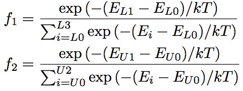 (Eq. 4.2.1)(Eq. 4.2.2)
where k is a Boltzmann constant, 1.38 x 10^-23 [J/K], T is temperature, Ei is energy at level i, respectively. The condition for the inverse distribution is expressed as follows.
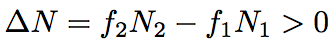 (Eq. 4.2.3)
When we have β, a rate of N2 to the total number of Yb3+ (N), the minimal pumping rate necessary for achieving the inverse distribution is shown as follows.
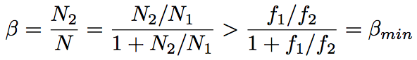 (Eq. 4.2.4)
βmin = 0 for a four-states system, βmin=0.5 for a three-states system. Fig. 4.7 represents βmin of Yb silica glass as a function of temperature. In order to obtain the inverse distribution at room temperature, approximately 5 % of Yb3+ must be exicted to the upper state. As the temperature decreases down to 100 K or lower, the minimal pumping efficiency decreases down to 0.02 % or less, then Yb silica glass laser can be seen as a four-states system.
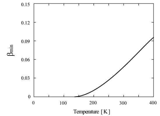
Fig.4.7 The minimal pumping efficiency necessary for achieving the inverse distribution
11.2 Er-doped fiber
Er-doped fiber is a three-states system. The typical pumping wavelegnth is 980 and 1480 nm, and the oscillation wavelength is around 1550 nm (see Fig. 4.4(b)). In the case of 980 nm pumping, compared with the case of 1480 nm pumping, the efficiency of power conversion from the pumping ligh to the signal light is lower, as well as the the width of absorption spectrum is narrower.
The gain coeffiicient of Er fiber is enlarged by increasing an amount of Er3+. However, as the Er concentration increases, the pumping efficiency decreases because of the concentration quenching. Er concentration for the quenching is, for pure SiO2 host, several hundreds wtppm. The Er concentration is increased when Al, which can suppress the concentration quenching, is co-doped into SiO2 host (Al2O3-SiO2 host), but is at most up to around 1000 wtppm. The effect of increasing Er3+ concentration on improving gain coefficient is limited. This limiation is made by a cooperative up-conversion between the ions. The cooperative up-conversion is the following phenomenon; provided that a couple of Er3+, excited to a 4I13/2, are close to each other, one of two Er3+ is excited to 4I9/2, while the other is deactivated to the ground state. The increase in the density of Er3+ cause the formation of Er3+ clustering, and then makes the distance between the ions closer, which yields the cooperative up-conversion. This process is schematically shown in Fig. 4.8(a).
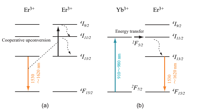
Fig.4.8 Schematic of energy transfer between ions on Er+3 ion
(a) up-conversion, (b) sensitization by Er:Yb co-doping
In an Er:Yb fiber where Yb and Er are co-doped, it is possible to improve the limitation of Er3+ doping concentration, which is a reason for the concentration quenching (suppression of concentration quenching). This is because the distance of Er3+ becomes long when Er3+ is surrounded by several Yb3+, of which radius is comparable with that of Er3+, and forms a cluster. The wide absorption band of Yb3+ is utilizable for the pumping wavelength.
Energy level diagram of Er:Yb is shown in Fig.4.8(b). After excited to the 2F5/2 level by 910-980 nm light, Yb3+ interacts with Er3+, then tramsfers to the ground state, 2F7/2, while Er3+ is excited to the 4I11/2 level (energy transfer). Er3+, excited to the 4I11/2 level, goes through a non-radiative decay, and is relaxed to the 4I12/2 level. As a result, the inverse distribution is formed between the 4I13/2 and 4I15/2 levels. The efficiency of energy transfer from Yb3+ to Er3+ largely depends on the doping ratio of Er3+ and Yb3+ and the core composition. An Er:Yb fiber, at 980 nm pumping, has a lower conversion efficiency (~ 45 %) compared with an Er fiber because of the complex process of energy transfer, such as Er-Yb transitions and parasitic oscillation between the levels in Yb.
FIg. 4.9 represents cross-sections of absorption and stimulated emission of Er3+ in the Er:Yb-doped phosphate glass as a reference.
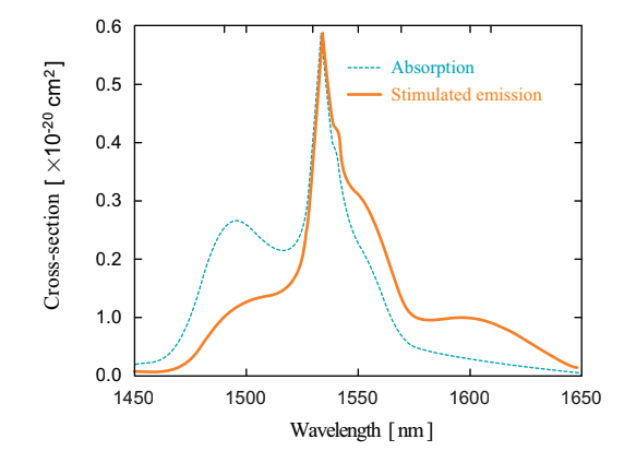
Fig.4.9 Absorption and stimulated emission cross-sections of Er+3 ion
12. Feedback device – Fiber Bragg grating
Fiber Bragg grating (FBG) is a fiber-type device, which has a periodic refractive index in the core of optical fiber. The periodic refraction works as a diffraction grating that reflects light of a particular wavelength satisfying the Bragg reflection condition. By using an FBG, a grating is formed in an optical fiber without destructing the fiber. An FBG is low-loss, compact, highly-reliable, and has a good matching property with transmission optical fibers. The schematic structure of FBG is shown in Fig.4.10.
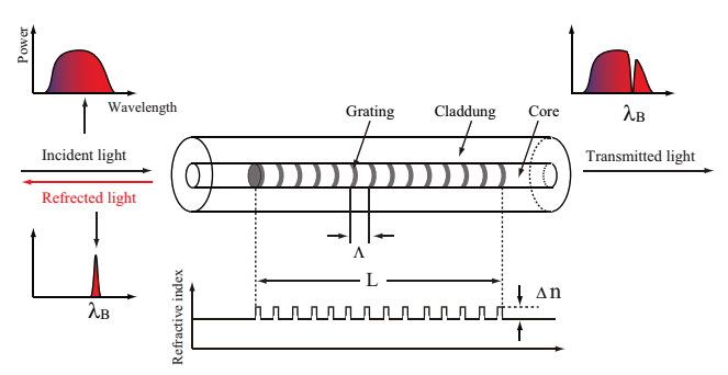
Fig.4.10 Fiber Bragg grating
A Fabry-Perot type fiber laser employ either of two feedback systems: one returns light with a lens and a mirror, as shown in Fig. 4.11(a), the other returns light with an FBG, as shown in the Fig.4.11(b). In the case using the FBG, a passive fiber with having the same diameter of core and clad as a gain fiber is employed, and is applicable to uses for a high-power fiber laser (a commercial product can be used for ~800 W output). Both of the feedback systems achieves the output 1kW or larger, while only an FBG can make the reflection range as narrow as ~0.1 nm.
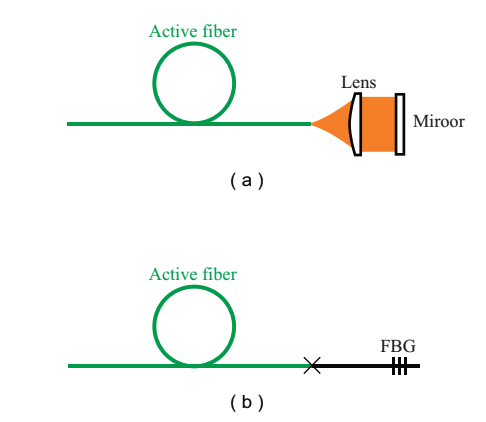
Fig.4.11 Return element of fiber laser
(a) space element, (b) FGB
Structure
As a function of grating periodicity in FBG, Λ, and an effective refractive index of propagating mode in an optical fiber, neff, a reflection wavelength, λB (Bragg wavelength), is expressed by the following equation.
![]() (Eq. 4.3.1)
(Eq. 4.3.1)
This relationship indicates that the the Bragg wavelength is arbitrarily tunable by chaning Λ. neff is represented by using a core refraction, ncore, and a refraction increment, Δn.
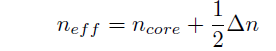 (Eq. 4.3.2)
A reflectivity at λB, Rb, and a reflecting range width, ΔB are expressed as follows,
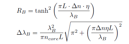 (Eq. 4.3.3)(Eq. 4.3.4)
where L is a grating length, and η is a rate of propagating wave in a core to total energy of propagating wave. The larger the grating length and the regraction increment are, the larger the grating reflectivity is (~99% in maximum).
An FBG is mainly useful for fiber sensor, though one is used for a feedback device in a fiber laser, and for selecting and stabilizing a laser wavelength. An FBG is applicable for measuring a strain and temperature change in a complex structure, because the wavelength of FBG is shifted in proportion to the strain and temperature. The wavelength of FBG for fiber laser is stable because a package for the temperature compensation is integrated in the FBG.
12.1. Manufacturing methods
When the core of an optical fiber doped with GeO2 is irradiated by UV laser in the wavelength of 223 ~ 253 nm, a photo-induced refraction change, caused by the change in Si-O bonding, occurs, and the refractive index semi-permanently changes. The amount of refraction change depends on the doping amount of GeO2 and the irradiation duration of UV laser. In an FBG, a periodic refractive index change is drawn by uses of interference pattern of UV laser.
Typical manufacturing methods are shown in Fig. 4.12 (a) phase mask method and (a) two beam interference method. As a UV laser, KrF excimer laser (248 nm), Argon ion SHG laser (244 nm), or Nd:YAG FHG laser (266 nm) is used.
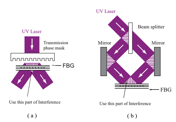
Fig.4.12 Manufacturing methods of fiber bragg grating
(a) phase mask method and (b) two beam interference method
In the case a refraction distribution in a whole grating has a homogeneous amplification in the direction of fiber axis, the reflection spectrum of FBG has a sidelope. When the refraction distribution is spindle-shape, a side lope can be depressed at 30~40dB or less. This is called as apodization. An FBG is also manufactured by using femtosecond laser instead of using UV laser.
(1) Phase mask method Phase mask method employs a penetrating phase mask having a periodic structure with a pitch of Λ/2 on quartz substrate, fabricated by electron beam lithography. When the phase mask is irradiated by UV laser, a pattern of interference between the plus and minus first-order diffracted light is yielded. The 0th-order can be minimized at less than several % by controling the depth and shape of grooves. Merits of the phase mask method are a reproducibility of FBG formation and to allow a use of low coherence laser. A weakness of the phase mask method is that the reflection wavelength is restricted to wavelengths inherent to the phase mask.
(2) Two beam interference method In two beam interference method, at fitst, UV laser light is split into two beam by a phase mask or beam splitter. Then, the split beam is directed and focused by mirrors, and an interference pattern is generated. This method is advantageous in freely setting the Bragg wavelength by controlling angles of the focused beam, but requres a highly coherent laser.
12.2. LPG and CFBG
A grating periodicity of typical FBG is around 1 µm. An FBG with a grating periodicity of several tenth ~ several hundredth µm is called long period fiber grating (LPG or LPFG). Different from the typical FBG, LPG does not reflect light, but radiate a clad mode to the outside due to a wide band range. An LPG is employed as an equivalent gain device of optical fiber amplifier. Because of a large periodicity, the interference is not necessarily used for manufacturing.
In some kind of FBG, a period of grating changes so that the low frequency components and high frequency components in a pulse are reflected at different positions. This is called as chirped fiber Bragg grating (CFBG). Fig.4.13 shows the schematic structure of CFBG. A CFBG is employed for the dispersion compensation and the pulse stretching.
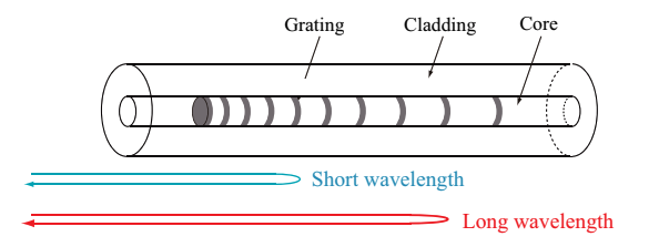
Fig.4.13 Structure of the chirped fiber Bragg grating
13. Optical isolator
In an optical isolator, light travels unidirectionally by preventing the light propagation in the opposite direction. A fraction of emitted light form a fiber laser return to the light source because of the reflections by optical componets such as optical connector terminals, objects, and lenses. The returned light can be a reason of laser power fluctuation and noise, and sometimes even break the light source. A slight amount of returned light is largely amplified in the fiber because the gain of fiber laser is very high. Therefore, the returned light can completely degrade a light seed or LD in the fiber laser, and the used optics. To avoid this issue, an optical isolator is necessary. In some cases, an optical isolator is integrated near a transmission fiber in the fiber laser or an input edge of the optical fiber amplifier.
An optical isolator is used in a ring-type fiber laser osciilator for a laser operation in the unidirection. A PM optical isolater, which is used for PM laser, also wokrs as a polarization control device,
Principle
In the operation of optical isolator, the Faraday effect, a magnetic optical effect where the polarization of light is rotated by the magnetic field, is employed. Faraday rotation device makes a linear polarization rotating. For communication uses (at 1250 nm or longer), bismuth, iron, and garnet (BIG), or yttrium, iron, and garnet (YIG) are employed. The device is very compact. In the wavelength from visible to YAG laser range (~ 1064 nm), terbium, gallium, and garnet (TGG) are used. TGG has a low Verdet constant, which determined the Faraday rotation angle. The optical isolator using TGG as the Faraday rotator requires several time larger magnetic power than the isolator using BIG, and is expensive. Types of an optical isolator is categorized into polarization dependent and polarization independent by its operation principle.
Polarization dependent isolator
As shown in Fig.4.14, rotating direction of the polarization is opposite between two cases: the magnetic field is applied to the Faraday rotator in the regular direction, or in the opposite direction (non-reciprocity). In the case of regular direction, a linearly polarized light produced by the polarizer A is rotated by + 45 degre by the Faraday rotator, and travels through the polarizer B, which is relatively tilted by + 45 degree to the polarizer A. In the case of opposite direction, because the polarization direction is rotated by – 45 degree, the polarization becomes orthogonal to the polarizer A, then the polarized light is blocked. This is the mechanism of polarization dependent isolator.
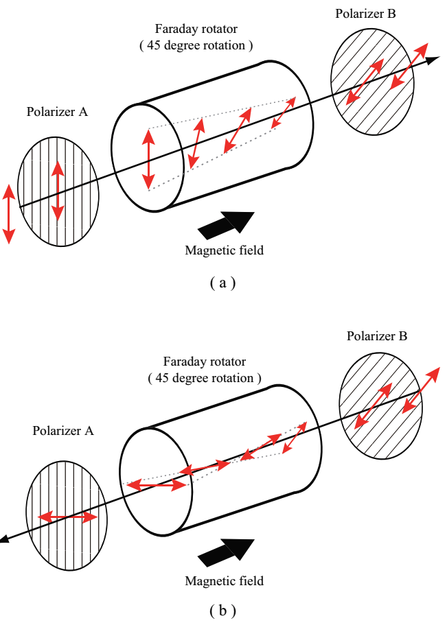
Fig.4.14 Mechanism of polarization dependent isolator
(a) the regular direction, (b) the opposite direction
The angle of polarization rotation by Faraday rotator, θ, is obtained by the following equation,
Eq. 4.4.1
where F is VErdet constant [minutes/oersted m], H is an axial intensity of magnetic field [oersted], and L is a length of Faraday rotator.
Polarization independent isolator
Polarization indenpendent isolator (or called as polarizatio insensitive isolator) devides linearly polarized light into an ordinary and extraordinary ray by using a birefringent crystal wedge instead of a polarizer. The devided rays travel as shown in FIg.4.15, and are merged into one at last. However, when light travels in the opposite direction, the devided rays are not merged. Although a typical system has a couple of collimator lenses and optical fiber at both edges of the birefringent crystal, the light travelling in the opposite direction is not focused at the optical fiber by the collimator lens. The polarization independent isolator can be used regardless of the condition of incident light, therefore is a general-purpose optical isolator.
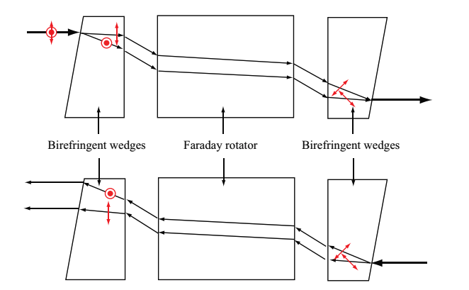
(1) Cautions An optical isolator is composed of intense magnets, the Faraday rotator, and polarizers. An attention needs to be paid for the fact that a magnet and Faraday rotator have a temperature dependence. Additionally, when an ultrashort pulse passes through an optical isolator, the pulse is dispersed by a device in the isolator, possibly resulting in pulse duration elongation by a factor of twice (@100fs).
The damage threshold of Faraday rotator is large: 20 kW/cm^2 for CW laser and 22.5J/cm^2 for 15ns pulsed laser, according to the test at 1064 nm for TGG from OFR Inc. The thresholding incident power for an optical isolator is mostly determined by polarizers. Polarizers can be film polarizers, polarized beam splitter, Glan crystal polarizers, or Brewster polarizers. For uses in a high power system, an absorption-type polarizer, such as a film polarizer, is not available.
13.1. Fiber optical isolator
In a fiber optical isolator, an optical isolator is equipped at the input and ouput edges of an optical isolator. For a polarization dependent isolator, because the operation depends on the polarization of incident light, PM fiber is employed (PM isolator). For a polarization independent isolator, both PM isolator and non-PM isolator can be utilized. The polarization independent isolator can be a PM isolator. A PM isolator does not allow the light travelling in the regular direction to pass except for polarized light along an axis (fast or slow) of the PM fiber
As a polarization independent isolator for integrated in an optical fiber system such as an EDFA and a fiber laser, an inline optical isolator is available. A typical inline optical isolator integrates a birefiringent crystal instead of polarizers, and is combined with an optical fiber.
Among performances of the fiber optical isolator, insertion loss, isolation, polarization dependent loss, polarization mode dispersion, and return loss are important. In case you bought the optical isolator, great attentions must be paid to a temperature dependence and a uniformity of each component besides the above-mentioned performances. By using a couple of isolators, the isolation can be 40dB or larger.
Items mentioned in the specification sheet of an optical isolator is explained below.
(1) Insetion loss A typically required value is approximately 0.6~1dB. When a low insertion loss is required, a requred value at the worst case is 0.5dB or lower for any temperature.
(2) Isolation An isolation has a wavelength dependence of polarization property. A required value is 30dB or larger for any wavelength range.
(3) Polarization dependent loss (PDL) A typical requirement for PDL value is 0.1~0.2dB for any temperature. Because the PDL can be accumulated, highly-demanded components are necessary for a multi-stage relay system.
(4) Polarization mode dispersion (PMD) A typical requirement for PMD value is 0.1ps. The requirement changes depending on a transmission speed of communication system. The required value is proportional to a square of the transmission speed. The PMD can be accumulated as well as the PDL, therefore, highly-demanded components are necessary for a multi-stage relay system.
14. Optical circulator
As shown in Fig.4.16(a), an optical circulator typically has three input or output ports. The signal light input into the port 1 is output from the port 2. The signal light input into the port 2 is output from the port 3. The optical circulator is often used with adding an FBG at the port 2 as shown in Fig.4.16(b). For reference, a composition of optical circulator is shown in Fig.4.17. Refer to a paper, regarding compositions and principles of compact optical circulators.
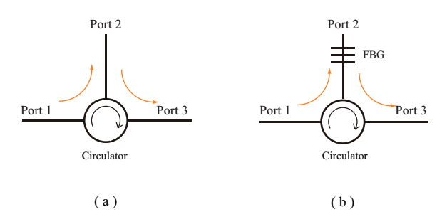
Fig.4.16 (a) Operation diagram and (b) usage example of the optical circulator
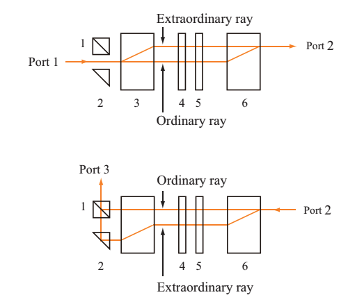
Fig.4.17 Configuration the optical circulator
1: Polarization beam splitter (PBS), 2: reflection prism, 3, 6: birefringent crystal, 4: faraday rotor, 5: 1/2 wave plate
An optical circulator is frequently used for an optical time domain reflectometer (OTDR), an optical add-drop multiplexer (OADM) and a dense wavelength devision multiplexing (DWDM) network using an FBG, and a pulse stretcher, a pulse compressor, and a disprersion compensator using a chirped FBG.
15. Mixing-wave device
An optical device for dividing optical power into two or more is called as an optical divider. A coupling device, which combines two or more optical powers into one, is called as an optical coupler. The optical divider is typically used as an optical coupler, when light is introduced into the divice from the rear side. Recently, an optical divider is also called as an optical coupler.
15.1. Category by structure
An optical coupler is categorized by its structure into a bulk-type, waveguide-type, and fiber-type (optical fiber coupler). Fig.4.18 summarizes the schematic of these three types of optical coupler.
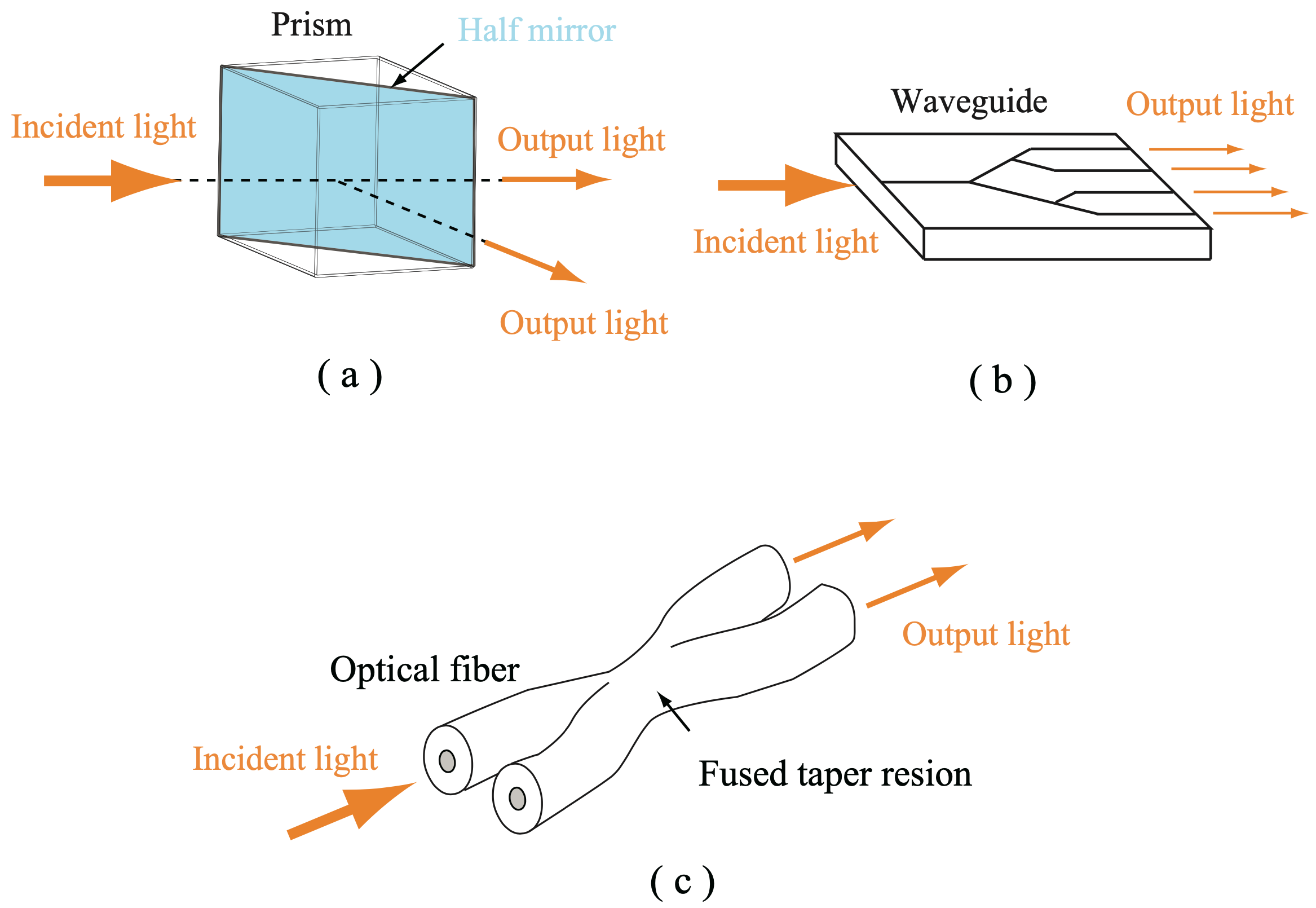
Fig.4.18 Types of optical coupler
(a) Bulk-type, (b) Waveguide-type (1:4), (c) fiber-type
(1) Bulk-type A bulk-type optical coupler is composed of small optical devices such as a half-mirror, beam-splitter, and filter. The division ratio can be changed by tuning the reflectivity at a plane of dielectric multilayer. This is advantageous in producing a wideband coupler. The bulk-type optical coupler has a larger insertion and is more expensive to produce loss than a fiber-type.
(2) Fiber-type A fiber-type optical coupler is manufactured by melting and extending a number of optical fibers, and is called as an optical fiber coupler. When a couple of optical fibers come close at the core, a mode coupling occurs, then, an optical power is divided into two, one of which is trasmitted to the other. By controlling the mode coupling length, an optical coupler with an expected division rate at specific wavelength can be produced, while a wideband coupler, and WDM coupler with a narrow wavelength interval is difficult to produce. Compared with the bulk-type optical coupler, the insertion loss and manufacturing cost are higher. The fiber-type optical coupler is used not only for the optical fiber communication, but also for a light source, monitoring optical fiber, exciting a fiber laser, an optical fiber amplifier, and a wavelength multiplexing system. The optical coupler with the division ratio of 1:1 is, in particular, called as the 3dB coupler, because it reduces the optical power into a half (-3dB).
(3) Waveguide-type A waveguide-type optical coupler manufactured by forming an optical circuit on a quartz substrate. Because a many-to-many optical coupler (waveguide-type coupler) can be collectively manufactured by the photolithographic technology, the waveguide-type coupler is advantageous in a mass-production and production cost.
15.2. Optical fiber coupler
An optical fiber coupler can be either of three types shown in Fig.4.19(a) splitting coupler, (b) wavelength division multiplexing (WDM), (c) combiner. In Fig.4.19, a Yb fiber laser is assumed, and the coupling or splitting wavelength is considered as 1030nm (laser light or signal light) or 980nm (pumping light) .
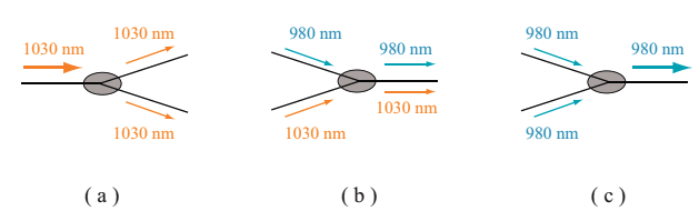
Fig.4.19 Types of optical coupler
(a) splitting coupler, (b) WDM coupler, (c) combiner
Splitting coupler
A splitting coupler splits light at a specific wavelength with a constant ratio, as shown in Fig.4.19(a), and is utilized as for distributing an optcal power of pumping and signal light and for monitoring the optical power. The splitting coupler is superior in the temperature controllability, producibility, and low cost. Required characteristics for the splitting coupler are a small error in the splitting ratio, a low excessive loss, and a low polarization maintaining loss (PDL). The details are described in the reference.
(1) Specialized splitting coupler In a wideband coupler, a wavelength dependence of splitting ratio is minimized, resulting in the flat splitting ratio at a wide wavelength range. The wideband coupler is employed in an interferometer for the optical coherence tomography (OCT) that uses a wideband light source such as a supercontinuum light. A star coupler is one of specialized splitting couplers, and is composed of a number of optical fibers, which are melted and combined in one. The star coupler allows a one-to-many splittingm therefore is the most important device for the optical LAN and optical access system.
15.2.1. WDM coupler
A WDM coupler splits or multiplexes multiple-wavelength light, as shown in Fig.4.19(b). The WDM coupler is used for multiplexing multiple-wavelength light input into specific different ports and outputting multiplexed light from a single port, or for splitting multiple-wavelength light input into a single port and outputting the split light from specific different ports.
15.2.2. Combiner
A combiner multiplexes light at a specific wavelength, as shown in Fig.4.19(c), and is often used for high power pumping. The combiner is either a polarization beam combiner or pumping combiner, depending on the core diameter. A polarization beam combiner is used for the strong pumping of a rare earth doped singlemode fiber, while an pumping combiner (pump combiner) is used for the strong pumping of a rare earth doped multimode fiber or double clad fiber. As to information on manufacturing processes of the combiner, see the reference.
(1) Polarization beam combiner A polarization beam combiner (PBC) is composed of polarization maintaining fibers as schematically shown in Fig.4.20. PBC achieves high power by superposing orthogonally polarized waves. PBC is required to be low loss, slight polarization crosstalk, and environment resistance. A slight temperature dependence of the optical property is also required. For a narrowband (within several nanometers range), a low loss combiner is relatively easy to manufacture, while it is difficult for a wideband (of several tenth nanometers range). Therefore, the usable bandwidth is limited.
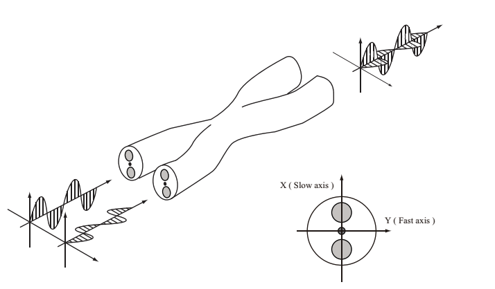
Fig.4.20 Structure of polarization beam combiner
(2) pumping combiner An pumping combiner is used in a high power (from several W to kW) CW fiber laser. The generated heat is integrated in CW laser, consequently a laser stability is distrubed. In order to remove the heat, the heat sink is equipped, and a measure of air-cooling or water-cooling is provided. A typical combiner is either Nx1 combiner or (N+1)x1 combiner as shown in Fig.4.21.
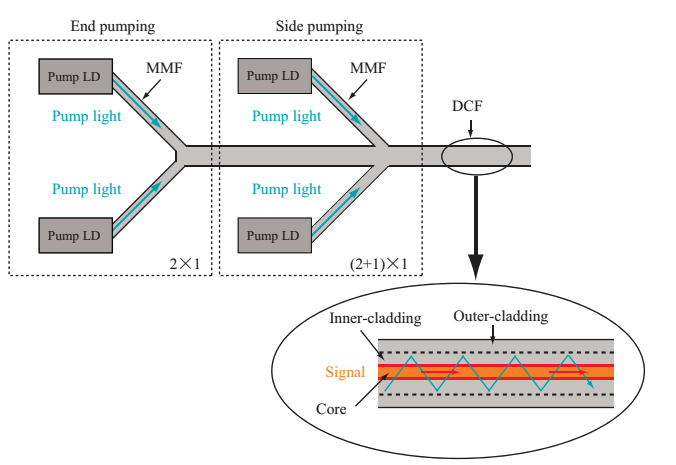
Fig.4.21 Nx1 combiner and (N+1)x1 combiner (N≧2)
In an Nx1 combiner, N of pumping fibers are combined in one. The Nx1 combiner is used for producing high power fiber laser oscillator and for combining a lot of rays without a large amount of signal light.
In an (N+1)x1 combiner, N of pumping fibers are combined in one, and a fiber for signal light is integrated. The (N+1)x1 fiber is used for producing a hIgh power fiber laser oscillator and hIgh power fiber amplifier. Commercially available combiners are mainly 2×1, 3×1, (1+1)x1, (6+1)x1, 19×1, and (18+1)x1.
16. Polarization controller
A polarization controller is composed of polarization control devices, such as a 1/4λ plate and 1/2λ plate. A fiber-type polarization controller modifies the elliptical polarization in an optical fiber to an arbitrary polarization. The fiber-type polarization controller can be either of three types, bulk-type, paddle-type, and inline-type.
(1) Bulk-type In a bulk-type polarization controller, as shown in FIg.4.22, light is once extracted from the optical fiber, and the polarization is controlled by using a bulk-type half-wave plate or 1/quarter-wave plate. The bulk-type polarization controller has a good controllability and thermal stability, but can have a coupling loss, therefore, an insertion loss can be high.
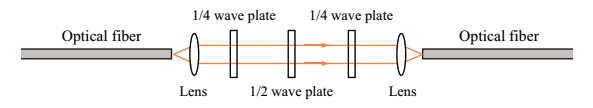
Fig.4.22 bulk-type polarization controller
(2) Paddle-type A paddle-type polarization controller is schematically shown in Fig.4.23; a paddle-type waveplate is formed by twisting an optical fiber round a coil, and the polarization is controlled by rotating each paddle. The paddle-type polarization controller utilizes a dependencies of optical fiber birefingence on the fiber diameter, fiber curvature, coil turns, and light wavelength. It is low-cost and low-loss, but a stability of polarization takes a time after a paddle controller is tuned.
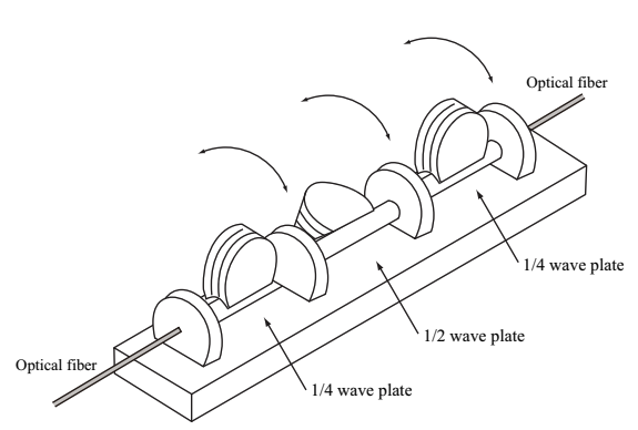
Fig.4.23 Paddle-type polarization controller
(3) Inline-type In an inline-type polarization controller, the polarization is controlled by pressuring and/or rotating an optical fiber with a knob as shown in Fig.4.24. The pressuring and rotation induces birefringence in the optical fiber, consequently the polarization is controlled. The inline-type polarization controller is compact and low-loss, but the pressure may cut an optical fiber.
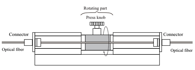
Fig.4.24 Inline-type polarization controller
17. Wavelength conversion element
A nonlinear optical crystal is a wavelength conversion element which extends the laser oscillation wavelength range to the infrared and ultraviolet. Generated light by using the nonlinear optical crystal has the same coherence as the laser fundamental line. For the wavelength conversion, a phase matching on birefringence of the crystal is necessary. Here, we consider the phase matching for the sum frequency generation (SFG). The SFG provides light with a sum frequency from light with two different frequencies. The relationship between the three wavelengths is expressed by the following equation according to the conservation law of light energy.
 (Eq.4.8.1)
By using the refractive indices of light, n1, n2, and n3, and a wavenumber, k=2πn/λ, according to the the conservation law of light momentum, the Eq.4.8.1 is rewritten as follows,
![]() (Eq.4.8.2)
(Eq.4.8.2)
This equation is the phase matching condition for SFG. The refractive index of crystal, n, is important; in other words, the absorption wavelength, dispersion, and birefringence of crystal is important. The refraction dispersion depends on the wavelength dependence. The approximate equation is the Sellmeier formula. If the polarizations of input light (λ1, λ2) were parallel, it is called as type I. If the polarizations are orthogonal, it is called type II. The phase matching condition is derived by using the anisotropy and dispersion of refractive index, and the conservatino laws of light energy and momentum.
17.1. Frequency conversion process
Here, other wavelength conversion processes, including SFG, is described. They are shown in Fig.4.25.
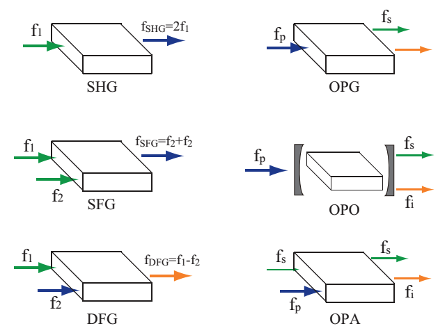
Fig.4.25 Wavelength (frequency) conversion processes
SFG generation
SFG provides high-frequency light from two kinds of low-frequency light as follows.
![]() (Eq. 4.8.3)
(Eq. 4.8.3)
SFG is employed for converting wavelength to the shorter.
e.g.) for 1064nm fundamental line
1064nm+1064nm → 532 nm: Second-harmonic generation (SHG)
1064nm+532nm → 355 nm: Third-harmonic generation (THG)
532nm+532nm → 266 nm: Fourth-harmonic generation (FHG)
1064nm+266nm → 213 nm: Fifth-harmonic generation (FIHG)
SFG generation
Difference frequency generation (DFG) provides light with a different frequency from two kinds of light with different frequencies as follows.
![]() (Eq. 4.8.4)
(Eq. 4.8.4)
DFG is employed for converting wavelength to the longer.
e.g.) 1064nm - 1550nm → 3400nm
Optical parametric generation
Optical parametric generation (OPG) provides two kinds of light with different frequencies from light with single frequency as shown below.
![]() (Eq. 4.8.5)
(Eq. 4.8.5)
OPG is a reverse process of SFG. Pump light (fp) is devided into signal light (fs) and idler light (fi). The change in an incident angle to the crysral can change the wavelength of generated light in a wide range.
e.g.) 355nm → 532nm - 1064nm
(1) Optical parametric oscillation Optical parametric oscillation (OPO), as OPG does, provides two kinds of light with different frequencies from light with single frequency as shown below.
![]() (Eq. 4.8.6)
(Eq. 4.8.6)
OPO is composed of a resonator with a couple of mirrors based on the OPG constitution.
(2) Optical parametric amplification In optical parametric amplification (OPA), the signal light is amplified by accepting energy from the pump light, and the idler light is generated simultaneously, when the signal light is provided with the strong pump light.
17.2. Phase matching method
For the wavelength (frequency) conversion, the phase matching condition must be satisfied. The phase matching is achieved by either (above-described) birefiringence phase matching (BPM) that uses birefringent crystals or quasi phase matching (QPM) which uses a crystal with periodically poled structure. The methods in BPM are, in principle, the adjustments of angle and temperature. The angle adjustment is the tuning of crystal axis to the the optical axis of incident beam. The temperature adjustment is the tuning of refractive index by the temperature control.
17.3 Crystal types
Wavelength conversion crystals have a dependency of availability on the wavelength and power of light. A crystal needs to be selected with comparing parameters such as refractive index, phase matching condition, effective nonlinear optical constant, and usable range, at used wavelength. In calculating these parameters necessary for high harmonic generation process, a nonlinear crystal program soft (provided by OptMax Inc. without charge) is useful. Typical crystals for the wavelength conversion are explained below.
KTP
KtiOPO4(KTP) is transmissive in the range of 0.35-4.5 µm. The mechanical strength, environment resistance, and optical damage resistance are good. Because the walk-off angle is small and the usable raneg of angle is large, KTP is useful for many uses. KTP is mostly used for SHG of Nd-doped laser oscilating at 1064nm, which is used as an pumping light source for titanium: sapphire laser. A walk-off angle is yielded from birefringence of crystal, and is defined as an angle bewteen incident and generated light in the crystal. The large walk-off angle means that the effective length of crystal, the area of nonlinear interaction bewteen incident and generated light in the crystal, is limited.
BBO
β - BaB2O4 (BBO) is transmissive in the range of 0.19-2.6 µm. The optical transparency and optical damage resistance are good. BBO is used for UV generation and high power solid-state laser. However, its birefringence is large. Therefore, the usable ranges of angle and wavelength are narrow, and the walk-off angle is large. Other drawback is the high hygroscopcity. BBO is employed for Nd:YAG laser FHG (266 nm) and FIHG (213 nm).
CLBO
CLBO is transmissive in the range of 0.18-2.7 µm. The optical transparency is good. CLBO is appropriate for a bulk system. The birefringence is relatively small compared with BBO. The usable ranges of angle, wavelength, and temperature are wide, and the walk-off angle is small. However, CLBO is brittle and hygroscopic. CLBO is used for ND:YAG laser FHG (266 nm) and FIHG (213 nm).
LN
LiNbO3 (LN) is transmissive in the range of 0.34-4.5 µm. The nonlinear optical property is good, and is used for both the bulk and waveguide types. LN tends to be optically damaged by the photorefractive effect. To improve the optical damage threshold, LN is doped with MgO.
For the phase matching of LN, both BPM and QPM is possible. Because LN is a displacement ferroelectric material, the polarity of LN depends on the application of electric field. The wavelength conversion by QPM for SHG is schematically shown in Fig.4.26.
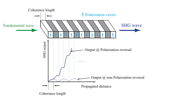
Fig.4.26 The wavelength conversion by QPM for SHG
As shown in Fig. 4.26, QPM utilizes the inversion of sign of nonlinear optical constant accompanied by the polarization inversion at each coherence length. QPM is called as periodically-poled LN (PPLN). By changing the period of inversion, the phase matching is acheived in the whole transmissive range, in other words, the phase matching condition can be satisfied at any wavelength. Although PPLN requires the temperature control, PPLN has a high efficiency and usability, and is used for varied applications. For instance, PPLN is employed for chirped pulse compression in case a chirped QPM grating is formed in PPLN. A chip-type PPLN is employed for the applications in mobile phone, laptop, compact projector, and in-car head-up display.
18. Optical fiber amplification
Optical amplifier is a name of the system in which optical signal is directly amplified without light conversion. Optical fiber amplifier, in particular, refer to the one employing an optical fiber as a gain medium. The optical fiber amplifier can be a rare-earth-additive fiber or an optical fiber Raman amplifier. The optical fiber amplifier was eagerly developed in 1980s, nowadays, is essential for the optical communications.
18.1. Rare-earth-additive optical fiber amplifier
In an optical fiber amplifier, the one employing Er fiber is called Erbium Doped Fiber Amplifier (EDFA), while the other using Yb fiber is named a Ytterbium Doped Fiber Amplifier (YDFA). The optical fiber amplifiers are generally composed of an pumping LD light source, a wave-mixer such as WDM coupler, optical isolaters, a rare earth additive optical fiber, as shown in Fig. 5.1. By removing the optical isolater and then incorporating loop devices, such as an FBG, at the edges of entrance and exit, the optical fiber amplifier becomes a Fabry-Perot fiber laser oscillator. The system of optical fiber amplifier is either of following three: forward-pumped type where the propagating direction of signal and pumping light are the same, backward pumping type where the propagating direction is opposite, and bidirectional pumping type where the pumping light is supplied from both a regular and opposite direction, as shown in Fig. 5.1 (a),(b), and (c), respectively.
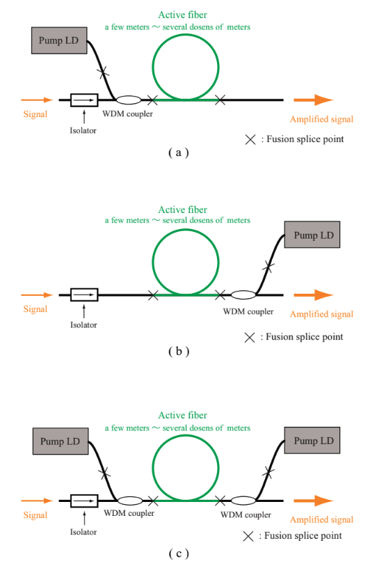
Fig.5.1 The basic configuration of optical fiber amplifier
(a) forward pumping system, (b) backward pumping system, (c) bidirectional pumping system
The optical isolator indroduced between input edge and gain fiber (see Fig. 5.1) plays a role of gain amplification by suppressing a parasitic oscillation (an unintentional or uncontrollable laser oscillation accompanying with a valid oscillation) and feedback of amplified spontaneous emission (ASE). The optical isolator is often also introduced between the optical fiber and output edge for the sake of higher gain.
Commercially available EDFA amplifies the signal in the wavelength region of 1530~1610nm. In general, the forward-pumped system superior in noise property uses the pumping light of the wavelength of 980nm, while the backward pumping system superior in output property uses pumping light of the wavelength of 1480nm. YDFA amplifies the signal in the wavelength region of 1030-1090nm. The wavelength of pumping light is 915 and 975 nm. In the communication range, a Thulium doped fiber amplifier (TDFA) for 1.45-1.5 and 1.67 µm range amplification and Praseodymium doped fiber amplifier (PDFA) for 1.3 µm range amplification are commerically available besides the EDFA for C band (1530-1565nm) and L band (1565-1625nm).
18.1.1. Noise in optical fiber amplifier
In the systems shown in Fig. 5.1, amplified signal may include a wide range spectrum, which is not a part of input light. This wide spectrum is an ASE. ASE is a dominant origin of the noise in the optical amplifier.
The main noises of optical amplifier are the following four:
1. Shot noise of amplified signal
2. Shot noise of ASE
3. Beat noise of ‘amplifeid signal’-ASE
4. Beat noise of ASE-ASE
A primary noise factor of laser light is the shot noise. The shot noise is originated from the quantum oscillation of light. The 3rd noise generates in the same range as signal, therefore, is not removable by optical filter, while the 4th noise can be removed by a narrow band filter. For the EDFA, removing the ASE in the range except for the signal range by inserting a narrow (1-3nm) band-pass filter behind the Er fiber improves noise property. The improved EDFA is then used for the optical communication. Regarding the 2nd noise, the stronger the signal is, the more noise is reduced. The stronger the signal is, however, the more remarkable the 3rd noise becomes. In the latter case, the 3rd noise is a primary noise factor.
A power ratio of signal to noise is denoted by S/N. S/N of input signal and amplified output signal gives a noise figure (NF) as shown below.
NF = … (5.1.1)
The unit of NF is dB. As the NF is small, the amplifier is a low-noise system. In an ideal amplifier where the inverse distribution is realized (N2>>N1), NF can be 3dB(quantum limit). Because the spontaneous emission necesarily generates, the ‘amplified signal’-ASE beat noise is always larger than zero. NF of EDFAs on the market are in the range of ca. 5~9dB.
18.2. Fiber Raman amplifier
Raman amplifier employs stimulated Raman scattering (SRS) for the optical amplification. Fiber Raman amplifier (FRA) employs an optical fiber in the Raman amplifier. FRA has advantanges in the optical communication for widening signal range and improving the transmission property. FRA is an inviting technology for high-capacity communication. A typical system of backward pumping FRA is shown in Fig. 5.2. FRA can apmlify output signal with awavelength ca. 100 nm longer than input signal. Because FRA has a wide gain range, an optional wavelength range is amplified when the pumping wavelength is tuned. This is why FRA is expected as a unique technology for solving the recent communication issues of the widening signal range and the increasing capacity. Raman amplifiers are also superior in the property of distribution-type amplifier because the amplification occurs with a low noise and spectral distribution in the long (several tenth kilometers) optical fiber where the pumping light can propagate. The drawback of FRA is a low amplification efficiency, then needs a sevaral kilometers long optical fiber.
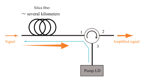
Fig.5.2 The configuration of Fiber Raman amplifier
18.3. Rate equation
A fundamental operation analysis will be shown by deriving simple rate equations from energy level of Yb silica glass. The sum of Yb3+ density in a ground and excited state (N1 and N2) equals the number of Yb3+ per unit volume (N).
 (Eq. 5.1.2)
The rate equation of steady state is expressed as follows,
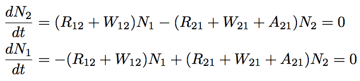 (Eq. 5.1.3)(Eq. 5.1.4)
where R12 and R21 are the pumping coefficients, W12 and W21 are the stimulated transition coefficients, and A21 is the spontaneous emission transition coefficient. These coefficients are obtained by follows,
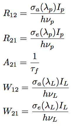 (Eq. 5.1.5)
where λP, and λL are the wavelength of pumping, and signal light, respectively, τf is a lifetime of spontaneous emission (fluorescence lifetime of laser medium), and σa, and σe is the cross-section of absorption and spontaneous emission. Eqs. 5.1.3 ~ 5.1.5 give N2 as follows.
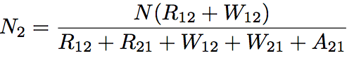 (Eq. 5.1.6)
18.4. Light propagation along the optical axis in fiber
By deriving an equation of light propagation in an optical fiber for forward- and backward-pumped system, shown in Fig. 5.3 (a), and (b), respectively, here we estimate a small-signal gain of optical fiber amplifier.
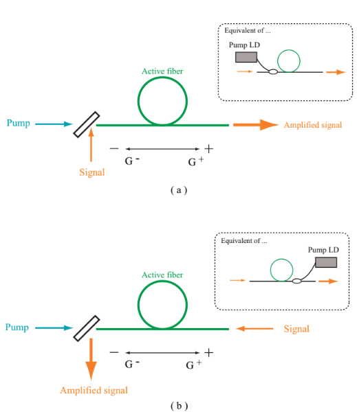
Fig.5.3 Schematic of (a) forward- and (b) backward-pumped system
When PL+, signal light propagating in the forward direction for pumping light in the forward-pumped system, and PL-, signal light propagating in the opposite direction for pumping light in the backward pumping system are given, propagation equations for signal and pumping light (Pp) along the optical axis of fiber are expressed as follows,
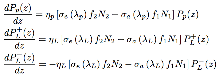 (Eq. 5.1.7)(Eq. 5.1.8)(Eq. 5.1.9)
where f1 is a Yb3+ ratio in L1 state to the ground state, and f2 is a Yb3 ratio in U0 state to the excited state. The first, and second term in Eq. 5.1.7 corresponds to a process that Yb3+ transfers to the lower state of laser medium by stimulated emission, and a process that Yb3+ is excited to the upper state. In the Eqs. 5.1.8 and 5.1.9, the first, and second terms correspond to the stimulated emission processes of signal light, and the absorption processes of signal light. ηp, and ηL means an overlapping rate of pumping, and signal light with fiber core, respectively. For a double-clad fiber, ηp, ηL is approximately Aco/Acl, 1, respectively, where Aco, and Acl is a cross-section area of fiber core and internal clad, respectively. Eqs. 5.1.7 ~ 5.1.9 enables numerical analysis of amplification gain and laser output power.
18.4.1. Small-signal gain of optical fiber
In order to analytically solve Pp(Z), we employ Eq. 5.1.7 and a following equation,
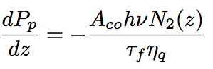 (Eq. 5.1.10)
where ηq is a pumping quantum efficiency, ~1 for Yb3+. Eqs. 5.1.7 and 5.1.10 give a following equation,
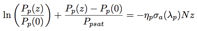 (Eq. 5.1.11)
where Pp(0) is exictation power at the input edge, and Ppsat is a pumping saturation power.
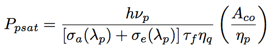 (Eq. 5.1.12)
Pp(z) is a calculated from Eq. 5.1.11. In general, Eq. 5.1.11 must be numerically solved for the calculation of absorption pumping power by optical fiber length. Provided Pp(0) << Ppsat, Eq. 5.1.11 is approximated as follows.
![]() (Eq. 5.1.13)
(Eq. 5.1.13)
Single pass gain for optical fiber length is expressed by a following equation.
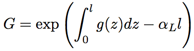 (Eq. 5.1.14)
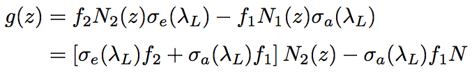 (Eq. 5.1.15)
where αL is a damping constant for laser siganl light.
The expression of small-signal gain is simplified by Eq. 5.1.10. Ppabs, a pumping power, that is absorbed by Yb fiber, is obtained from Eq.5.1.10.
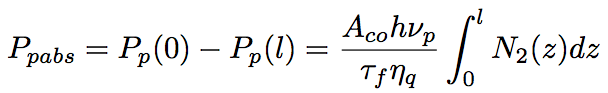 (Eq. 5.1.16)
In summary, the small-signal gain, G, is obtained as follows.
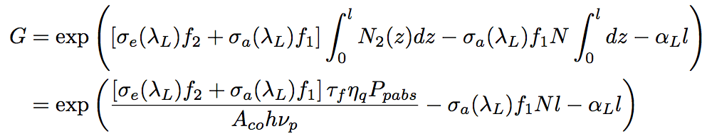 (Eq. 5.1.17)
The second, and third term explains a reabsorption loss, and a propagation loss of fiber core. When the small-signal gain, G, is converted to dB expression, fiber gain is obtained.
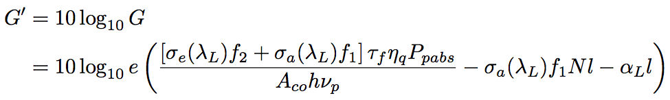 (Eq. 5.1.18)
(1) Clad pumping Yb fiber amplifier
We consider a clad pumping Yb fiber amplifier. Provided the core diameter =10 µm, h = 6.63 x 10⁻³⁴ Js, τf=1ms, λp=975nm, λL=1064nm, σe(λL) ~2.82×10^-25m^2, f1=0, f2=1, σe(λL)~0, and the propagation loss αL~0 (under the assumption of four states in long wavelength range), the gain characteristics against absorption pumping power is obtained as shown in Fig. 5.4. The practical small-signal gain is 30~40dB owing to a parasitic oscillation and and ASE in the optical fiber.
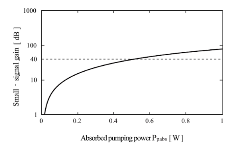
Fig.5.4 The gain characteristics against pumping power of clad pumping Yb fiber amplifier
(2) Core direct pumping Yb fiber amplifier
We consider a core pumping Yb fiber amplifier. Provided the core diameter =6 µm, τf= 1ms, ηq=1, λp=975nm, N=9.5×10^25m^-3, l=1 m, and σL ~ 0, the gain characteristics against signal wavelength, G'(λL), is obtained as shown in Fig. 5.5. The pumping absorption power, Ppabs, is changed between 0 and 70 mW. For the larger pumping power, the peak wavelength of output light is red-shifted, because the practical small-signal gain is 30~40dB.
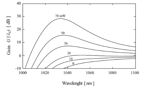
Fig.5.5 The gain characteristics against wavelength of direct core pumping Yb fiber amplifier
18.4.2. Comparison between forward- and backward-pumped systems
Table 5.1 compares forward- and backward-pumped systems shown in Fig.5.3. For the backward pumping system, the inverse distribution efficiency is low because of the damping of pumping light in the vicinity to the edge of signal light input. However, because spontaneous emission light is accumulated in the axial direction even for N2=N1 (transparent condition), the noise to signal ratio becomes integrated.
Table 5.1: comparison of forward- and backward-pumped systems
| Foreward-pumped system | Backward-pumped system | |
| Noise Factor | low | high |
| Power | low | high |
| Nonlinear optical effects | high | low |
| ASE | small | many |
For the forward-pumped system, on the other hand, though the noise by spontaneous emission exists as well, the signal light is also amplified because the inverse distribution is remarkable enough in the vicinity to the edge of signal light input. Therefore, noise factor (NF) does not change. Thus, because the forward-pumped system is superior in the noise property, it is proper for the use as a pre-amplifier which requests for low-noise property, while the backward pumping system is appropriate for the use as a power-amplifier because of its excellent output characteristics.
For the power amplification, the backward pumping system is better because of G+=G- in the small-signal gain range and G+
Eq. 5.1.19
PLsat ~ 52 mW for the case shown in Fig.5.4. For the sake of efficient power extraction in the light amplification, input light stronger than the saturation power is necessary.
19. Chirped pulse amplification (CPA)
In laser with small saturation fluence and short upper-state lifetime, such as excimer and dye laser, nonlinear optical effects such as self-focusing barely occur, while On the other hand, in laser with large saturation fluence such as solid-sate laser, the destruction of laser medium (threshold intensity: 1×10^10 W/cm^2) restricts the peak power of a pulse. Chirped pulse amplification (CPA) in which a chirp is controlled has been developed to .overcome the destruciton issue. CPA has dramatically improved the laser peak output. CPA has realized the PW-class (10^15 W) peak output laser system. CPA is applicable to the parametric amplifier (named optical parametric chirped-pulse amplification (OPCPA)).
5.2.1 System configuration
The system configuration of CPA is shown in Fig. 5.6 and explained as follows.
(1) The system of CPA requires a mode-lock laser oscillator for the stable generation of ultrashort pulses. (2) A output pulse from the ultrashort pulse laser oscillator is linearly chirped by a pulse stretcher, consequently the pulse duration is elongated, which realizes the suppression of peak intensity. The chirping is realized by medium dispersion by the propagation material, angle dispersion by geometric optical path differnence, which can be brought by a pair of rebulk-type diffraction grating, or other types of dispersion, such as a dispersion brought by the nonlinear process of self-phase modulation in an optical fiber. The dispersion measure is defined as GVD. (3) Pulse energy is amplified before the peak intensity exceeds the optical destruction threshold of the amplifier medium. (4) A pulse compressor shortens the pulse duration by giving GVD of which sign is the opposite to that of GVD given by the pulse stretcher to the pulse. The pulse compressor is typically a pair of diffraction grating. In theory, the pulse duration is compressed as it was before the pulse stretching.
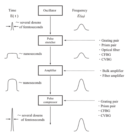
Fig.5.6 The configuration of CPA system
The pulse stretcher is typically a bulk-type diffraction grating or optical fiber. It elongates the duration of ultrashort pulse by 10^3~10^5. Provided that the pulse is stretched from 100fs to 1ns (by 10^4), though, the grating pair needs the wide space and its configuration is complicated. The fiber does not require such a wide space because it can be rolled, but it needs a long wire (~1km), consequently suffers from the loss. As a better pulse stretcher, Chirped fiber Bragg grating (CFBG) is recently developed. In CFBG, the reflection region is different between low and high frequency components in a pulse. CFBG with the approximate length of 10 cm can elongate a 100 fs pulse up to 500 ps. CHBG is a compact, and suppresses the loss and nonlinearlity. A recent report presents a CPA with using chirped volume Bragg grating (CVBG) as the stretcher and compressor. CVBG is a compact and surpasses in the optical resistance, the environmental characteristics, and the thermal stability, because the grating is crystallized inside the glass.
(1) Fiber CPA system Fiber charped pulse amplification (FCPA) configurates CPA laser system with optical fiber. Femtosecond FCPA recently achieved 12 MW peak power and 830 W average output with 640 fs pulse duration and 78 MHz repetition rate at 1042 nm center wavelength.
Fig. 5.7 shows a system configuration of the high peak power and output laser as an example of FCPA. Different from the above-mentioned CPA, a negatively chirped pulse (down-chirp) generated by CFBG is first amplified, and then is compressed by transmitting through a positive dispersion medium such as a glass block (called as fIber down chirped pulse amplification: FDCPA). Because a pair of bulk-type diffraction gratings is not employed for the pulse compression, the optics is simple.
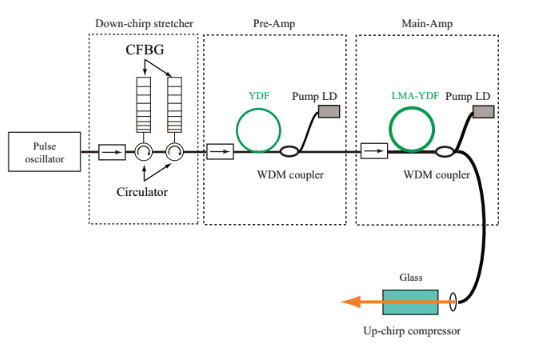
Fig.5.7 The configuration of the high peak power and output laser with the fiber down chirped pulse amplification
20. Master oscillator power amplifier (MOPA)
In master oscillator power amplifier (MOPA),a stable master oscillator (or a light source) generating high-grade beam and a high power optical amplifier are separately controlled. MOPA is featured by the good beam property and high output power. MOPA laser system is often used for high power applications such as laser micro-processing. FIg. 5.8 shows a schematic configuration of MOPA system. Master oscillator (MO) can be an LD, fiber laser, or bulk-type solid-state laser. The oscillation type can be low power CW, pulse (Q-switching), short pulse, etc. As an optical amplifier, a set of optical fiber amplifiers, called fiber MOPA or master oscillator fiber amplifier (MOFA), is typically employed in order to obtain high power output in MOPA, while bulk-type is also sometimes used. In the optical fiber amplifier, the core diameter of gain fiber (such as a large-mode-area double-clad fiber: LMA-DCF) is larger for the output side compared with the input side, as well as the pumping intensity. The optical fiber amplifier often requires the use of band-pass filter between the amplifers to minimize the ASE.
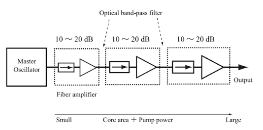
Fig.5.8 The configuration of MOPA system
A stable fiber MOPA without a valid connection loss can be configurated if fiber pigtail LED or fiber laser is used as a master oscillator. Fig.5.9 shows an example of MOPA fiber laser configuration.
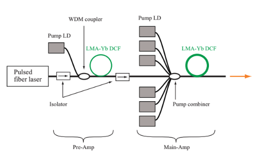
Fig.5.9 The configuration of MOPA fiber laser
21. Beam quality
In a typical manner, laser beam quality is evaluated by M^2 factor. In the notation using M^2 factor, higher-order transverse mode light is considered as Gaussian beam of which spot diameter is as M times large as that of fundamental tranverse mode light. The divergence angle of beam focused by lens is M^2 time larger for higher-order transverse mode light compared with the fundamental transverse mode light. For M^2=1, a beam spot corresponds to a fundamental Gaussian beam.
Fiber laser osicllation can be done with fullly single transverse mode (LP01 mode) provided that the optial fiber and fiber-type components configurating the oscillator are all single-mode types. Therefore, the fiber laser can achieve a theoretical limit of output beam quality, M^2=1. Because of this, the fiber laser is thought as an extremely small laser light source, and is appropriate for the use on laser marking which demands a good technique of miniaturization.
LMA fiber can achieve a good beam quality close to the single mode beam, despite a large bore fiber, because mode filtering effect works when the bending loss is applied. Without a compelling mode-lock, the beam quality M^2 for core diameter and NA is obtained by the following equation.
where d is the core diameter, NA is the core aperture, and λ is the wavelength of the incident light. Figure 5.10 shows the limiting value of M2 for core diameter when λ = 1064 nm and NA = 0.075.

22. Optical destruction threshold for optical fiber
One of the disadvantages of fiber laser oscillator is that the edge section if optical fiber tends to be damaged. This is because the quartz glass, main mateiral composing the core, has a lower damage threshold compared with laser crystals such as YAG, and also because the power density is very high at laser medium, the edge section of the core in a diameter of 10 µm. Furthermore, when the fiber laser is used for laser processing, which deals with high-power laser, the reflection light on the processing area may possibly destroy the laser output part.
The optical destruction of optical fiber often occurs owing to a parasitic oscillation accompanied by Frenel reflection at the edge section. The parasitic oscillation is effectively suppressed by cutting the edge face at a diagonal line as shown in Fig. 5.11(a). A fiber cleaver for the diagonal cutting is commerically-marketed.
But silica glass fibers doped with rare earth ions have a lower damage threshold compared with undoped silica glass fibers. Therefore, recently, a coreless undoped silica glass fiber is fused at the edge of rare earth doped fiber (End-cap system). The optical destruction at the fiber edge face is minimized because the most of Frenel reflection light by the edge face is guided to the clad. Endcap system is applicable to the photonic crystal fiber. One practical problem is the fact that light is collected at the fiber edge section. Because the edge section pumping is empirical, a reliable pumping method should be developed for industrical high power fiber laser.
When an edge section of optical fiber is damaged, the damaged volume needs to be cut out. Subsequently, the fiber will be in use again. When the inside of fiber is damaged, the damaged volume must be cut out, and the intact parts of fiber need to be connected by the fusion splicing method for reuse. However, a slight loss of fusion splicing can yield a lowering of the optical destruction threshold, and localized light scattering and laser oscillation in a high power fiber laser. This makes the reused fiber unreliable in a long term. The optical damage of fiber occurs not only at a local region, but also runs along the fiber. This phenomena of melting destruction is called “fiber fuse.”
In the following sections, the optical damage threshold for CW and pulsed laser oscillation is discussed.
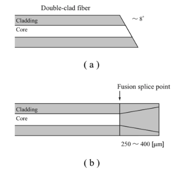
Fig.5.11 The methods for suppressing the edge section reflection
Schematic of (a) cutting the edge face at a diagonal line, (b) connecting endcap
CW oscillation laser
The optical damage threshold at silica glass surface of bulk-type fiber is 2 GW/cm^2 for CW or high-repetition pulsed oscillation, while the damage threshold is approximately 1 GW/cm^2 for rare earth doped silica glass. Provided that the optical damage threshold is 0.5 GW/cm^2, output limit characteristics against mode raidius is obtained as shown in the Fig.5.12. The optical damage threshold, 0.5 GW/cm^2 was estimated under the assumption that light propagates through optical fiber with the Gaussian distribution in space. Under the assumption, the light energy is focussed in the core center. Note that heat given by the pumping light is not considered for the output limit. Fig. 5.12 also shows SRS and SBS threshold, given by the following equations.
 (Eq. 5.5.1)
We assume the followings: the beam is single mode, Raman gain coefficient (gR), and Brillouin gain coefficient (gB) is gR ~ 1.2 x 10^-13[m/W], gB ~ 2.0 x 10^-11 m/W, respectively, and the effective interaction length of optical fiber (leff) is 5 m. Fig.5.12 means that the damage of high-power fiber laser with CW oscillation is determined by SBS.
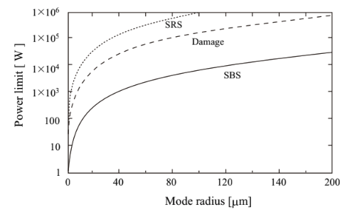
Fig.5.12 Output limit characteristics at an effective interaction length of 5 m for an optical fiber
Pulsed oscillation laser
The optical damage threshold at bulk-type silica glass is appoximately 50 J/cm^2 for 1ns duration pulse. Fig.5.13(a) shows the optical damage threshold of optical fiber with the core diameter of 10µm, 30µm, 100µm, and 200µm at 1ns duration pulsed laser irradiation. Fig.5.13(b) shows the damage threshold for 10µm core diameter in detail. Because the optical damage threshold for pulsed oscillation is determined by both the threshold of bulk and self-focusing effect of silica glass, a type of Kerr effect where the beam is focused at single point in the medium, the intensity threshold of self-focusing is also presented in the figures. The self-focusing threshold of silica glass is 3.7 MW, which is derived from the nonlinear refractive index (n2: 2.2 ~3.4 x 10^-20 m^2/W). The pulse duration dependence of the bulk damage threshold follows the square-root law, in which as the pulse duration becomes longer by the multiplication factor of “x”, the damage threshold is improved by the multiplication factor of root “x.”
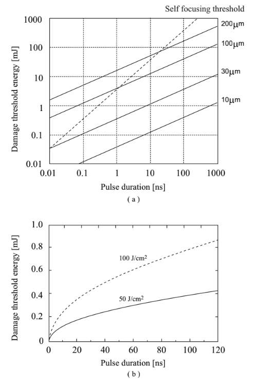
Fig.5.13 The optical damage threshold at 1ns duration pulsed laser irradiation
The optical damage threshold for the optical fiber with the core diameter of (a) 10µm, 30µm, 100µm, and 200µm, (b) 10µm
23. Thermal analysis for optical fiber
23.1. Thermal load limit
For the high average output laser, accumulated heat by pumping light in the laser medium can cause a problem. It is relatively easir for fiber laser to exhaust heat because the ratio of surface area and the volume is larger compared with rod-type, slab-type, and thin-disk-type solid-state laser. The thermal effect in optical fiber can cause its melting and optical damage, and spectral distortion by a temperature increase. Once thermal gradient is generated by an inappropriate treatment of heat release, a distortion of beam quality, which is caused by thermal lensing effect or thermal birefringence effect, and thermal destruction occur. A heating effect on the optical devices existing the outside, such as a Faraday-isolator, influences the operation of laser system.
Heat accumulated in the laser medium is principally generated by quantum defect, which is expressed by the following equation,
![]() (Eq. 5.6.1)
(Eq. 5.6.1)
where vp, vL denotes the frequency of pumping light, signal light, respectively. Another heating source can be excited-state absorption (ESA). ESA does not affect Yb3+ fiber, because Yb3+ is two-states system.
Pumping light is partly absorbed by dopant, and is converted to heat. The conversion ratio is give by the following equation,
 (Eq. 5.6.2)
where λp, λL is the wavelength of pumping light, signal light, respectively. γh is 0.05 ~ 0.20 (λp: 915~980 nm, λL: 980~1140 nm) for Yb3+.
Double-clad fiber
Fig.5.14 shows a schematic of end-pumping for double-clad fiber (DCF). The following discussions will be based on this figure.
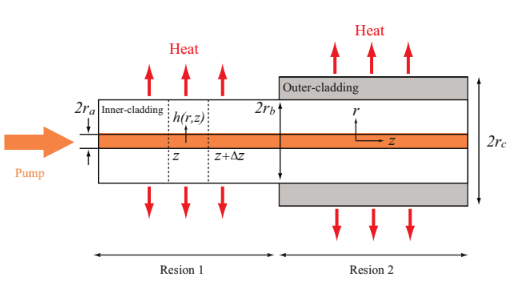
Fig.5.14 Schematic of end-pumping for double-clad fiber (DCF).
Heat value going through a cross section of a medium, h, is proportional to the gradient of temperature, T.
![]() (Eq. 5.6.3)
(Eq. 5.6.3)
Kc is a thermal conductivity of material (W/(mK)). In the steady state, the divergence of thermal flow is equivalent to the heat volume density.
![]() (Eq. 5.6.4)
(Eq. 5.6.4)
Assuming that the heat generated at the core of optical fiber radially flowed, the overall value of thermal emission from the volume between z and z+Δz is expressed as follows.
 (Eq. 5.6.5)
Therefore, the heat value, h(r,z), is expressed by the following equations,
") (Eq.5.6.6: inside the core)(Eq.5.6.7: outside the core)
(Eq.5.6.6: inside the core)(Eq.5.6.7: outside the core)
where Pp(z)=Pp(0)exp(αpz) is a pumping power at an axial position, z, and αp is an absorption coefficient of the pumping light at the core, in which rare earth ion is doped .
Assuming that the thermal conductivities of core and internal clad are the sameg, we have K=Kic (thermal conductivity of core and internal clad) for r<rb, and K=Koc (thermal conductivity of external clad) for r>rb. Under this assumption, temperature distribution is given by the following equation.
 (Eq. 5.6.8)
As we have Ts, a temperature around the optical fiber, the temperature distributions in the area 1 and 2 are expressed as follows.
![]() (Eq. 5.6.9)
(Eq. 5.6.9)
![]() (Eq. 5.6.10)
(Eq. 5.6.10)
In these two equations, Ph(z)=Pp(z)αpγh is an amount of heat generated per unit length, T(0,z) is temperature at the core center, and H1, and H2 is a coefficient of heat transfer between internal and external clads in the area 1, and 2, respectively. Provided that the thermal load limit is the melting point of silica DCF, a maximum thermal volume per unit length, Phmax, for the area 1, and 2 is expressed as follows.
 (Eq. 5.6.11)(Eq. 5.6.12)
Tm is a melting temperature of core of silica fiber. The 3rd term of Eq. 5.6.9 indicates for the area 1 that heat is efficiently exhausted for larger internal clad diameter, rb, due to the larger surface area. The 3rd term of Eq. 5.6.10 indicates for the area 2 that temperature is hard to increase for thinner external clad, rc, in the condition of Koc<<Kic.
Fig. 5.15 shows Phmax as a function of H in the area 1, and 2 for the following specifications of typical double-clad silica fiber.
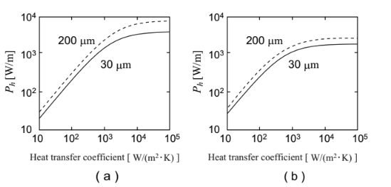
Fig.5.15 thermal load limit for heat transfer coefficient of double-clad silica fiber with core diameter of 10µm, 200µm
Heat load limit in the (a) area 1 and (b) area 2
① Core diameter 30µm, internal clad diameter 400µm, external clad diameter 550µm
② Core diameter 200µm, internal clad diameter 600µm, external clad diameter 800µm
We assumed Tm~2000K(1726.85℃) for silica glass, Ts~293K(19.85℃), Kic~1W/(mK) for silica internal clad, and Koc~0.1W/(mK) for polymer external clad.
When we assume H~10W/(m^2K) for spontaneous air-cooling and H~1000W/(m^2K) for water-cooling, a thermal load allowable in the area 2 of double-clad silica fiber with 30 µm core diameter for air-cooling, and water-cooling is Ph~30W/m, and Ph~1000W/m, respectrively. In reality, the thermal load limit is lowered because the melting temperature, Td, of polymer coating for the external clad in the area 2 is 150 ℃. With this consideration, Phmax is give as follows.
 (Eq. 5.6.13)
Fig. 5.16 shows the thermal load limit for coefficient of heat transfer of double-clad fiber with core diameter of 30 µm, and 200 µm under the consideration of mealting temperature of the coating. Optical fiber for high-power laser requires an effecitve heat exhaust. In order to increase a thermal load limit, an increase in the coefficient of heat transfer by cooling (such as water-cooling) is necessary.
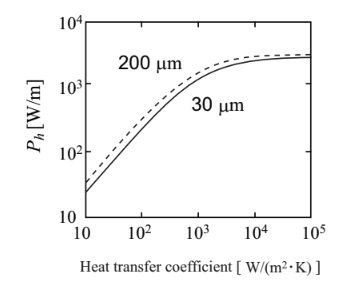
Fig.5.16 Thermal load limit for heat transfer coefficient of double-clad silica fiber with thermal load limit core diameter of 10µm, 200µm under the consideration of mealting temperature of the coating
Upper limit of extractable power
An upper limit of extractable power from the rare earth doped fiber is determined by the following equation.
 (Eq. 5.6.14)
For Yb fiber laser, where γh~0.1, Pmax~10Ph is obtained.
23.2. Heat distribution at DCF cross-section
In rare earth doped fiber, absorped pumping light is partially converted to heat. The generated heat can be released toward the outside by air-cooling and water-cooling. Steady-state temperarure at a distance of r from the center of heating medium, T(r), is obtained by the following heat conduction equation.
") (Eq. 5.6.15)
(Eq. 5.6.15)
where Kc is a thermal conductivity [W/(mK)], Q is a heat generation density [W/m^3]. Q is derived from heat value [W/m] and core cross section area [m^2]. Provided the thermal conductivity of internal clad, and external clad is Kic~1[W/(mK)], and Koc~0.1[W/(mK)], respectively, a temperature increase at cross-section of the following two types of DCF was numerically analyzed.
① Core diameter 30µm, internal clad diameter 400µm, external clad diameter 550µm, generating heat 7W/m
② Core diameter 200µm, internal clad diameter 600µm, external clad diameter 800µm, generating heat 60W/m
Fig. 5.17 (a, and b) shows the result of (1, and 2), respectively. The temperature increase at the core is 4.3 K (for ①) or 30 K (for ②). Both results show a dramatic temperature decrease at a part of external coating, indicating that the thinner external coating is effective for the heat release.
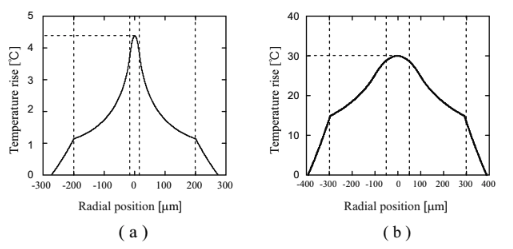
Fig.5.17 Temperature increase at cross-section of fiber
Temperature distribution at the core diameter of (a) 30µm and (b) 200µm
23.3. Heat stress in optical fiber
Heat exhaust is easy for optical fiber because the aspect ratio (length/diameter) is large. However, when the exhaust yields thermal gradient in the fiber, heat stress is applied. This section describes the heat stress of optical fiber in the elastic region where the fiber distortion can be spontaneous recovered.
The optical fiber length, L, is far larger than the internal clad diameter, 2rb (L>>2rb). In this condition, the heat stress at fiber cross section in a radical direction σr(r) and tangential direction σφ(r) is expressed by the following equations,
 (Eq. 5.6.16)(Eq. 5.6.17)
where α is a linear expansion coefficient, E is Young’s modulus, v is Poisson ratio (lateral stress[%]/axial stress[%]) in the elastic region. Heat stress at cross section of optical fiber, σz(r), is shown as follows.
![]() (Eq. 5.6.18)
(Eq. 5.6.18)
For the maximum value of σz (σmax), thermal shock coefficient, Rt, is given below.
 (Eq. 5.6.19)
Thermal volume density at thermal damage limit, Phmax, is expressed by the following equation.
 (Eq. 5.6.20)
Thus, the heat stress is evaluated by the thermal shock coefficient, Rt. Rt is independent of medium radius as long as the shape of laser medium is rod-type, therefore, is determined by a types of medium regardless of fiber or bulk. For silica glass (Kic=1.38 W/(mK), σmax=150MPa, Poisson ratio ν=0.17, α=0.55×10^-6K^-1, E=72GPa), Rt~4300W/m is obtained. Compared with the other bulk-type crystal and glass (Rt~1100, 3400, 100W/m for YAG crystal, Sapphire crystal, phosphate glass, respectively), the thermal shock coefficient of silica glass is larger. Silica glass surpasses in the thermal tolerance.
23.4. Thermal lensing effect in optical fiber
Thermal lensing effect is a phenomenon of refractive index change due to a local temperature increase in the medium caused by laser irradiation. The induced refractive index distribution, n(r), is expressed as follows (“th” means “thermal”, but not “threshold”),
 (Eq. 5.6.21)(Eq. 5.6.22)
where Kc is a thermal conductivity of material, Ph is a heat accumulation density. The thermal lensing effect is either that the temperature differentiation of refractive index (dn/dT) is positivem then a mateiral becomes a convex lens, or that dn/dT is negative, then a material becomes a conacve lens. dn/dT is negative for phosphate glass, therefore the phosphate glass diverges collimated beam. dn/dT is positive for silica glass, therefore silica glass focuses collimated beam. The thermal lensing effect causes degradation of beam property.
For the bulk-type solid-state laser, heat is integrated via its continuous operations. The integrated heat can cause the thermal lensing effect, which affects the laser optical path. When a laser medium is glass that has a low thermal conductivity, in particular, the thermal lensing effect is opt to be remarkable.
For an optical fiber, the thermal lensing effect also occurs, although is not so remarkable because its heat release property is excellent. Here, the thermal lensing effect in optical fiber is discussed.
Fundamental mode radius, w0, for SI-type fiber is expressed as a function of fiber core diameter, ra, and V parameter.
 (Eq. 5.6.23)
A mode radius affected by the thermal lensing effect is shown as follows.
 (Eq. 5.6.24)
For wth<wo, the thermal lensing effect influences the beam. Therefore, the heat accumulation density, Ph, is expressed as follows.
 (Eq. 5.6.25)
Provided V=2.4 (fundamental mode), no=1.45, Kc=1W/(mK), dn/dT=11.9×10^-6 K^-1, and λ=1064nm, generating power of the thermal lensing for the core radius is obtained as shown in Fig. 5.18. A thereshold of the thermal lensing effect is 140, and 3.2 W/m for the core diameter of 30, and 200 µm, respectively. The thermal lensing effect is not a serious problem when the core diameter is small because the thermal gradient is little. However, the thermal lensing effect is a remarkable issue for a fiber with large diameter and short legth. Effective improvements of the heat release method such as using a long fiber and cooling the fiber will achieve more reliable high-power fiber pulse laser.
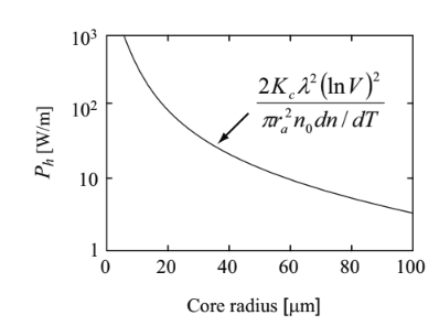
Fig.5.18 The volume density of generating power of the thermal lensing for the core radius, provided V=2.4 (fundamental mode), no=1.45, Kc=1W/(mK), dn/dT=11.9×10^-6 K^-1, and λ=1064nm